How to read these slides?
 Overview
Click on the menu bar items to navigate to chapters
Click here for PDF version (Note: No videos in the PDF version)
VU Fundamentals of
Geometry Processing
Marching Cubes
Julian Rakuschek
19.03.2026
In this lecture
How do we get from a symbolic equation $x^2 + y^2 + z^2 = R$ ...
... to a triangular mesh?
All about converting from implicit to explicit via marching cubes!
Supplemental Paper Reading

Introduction
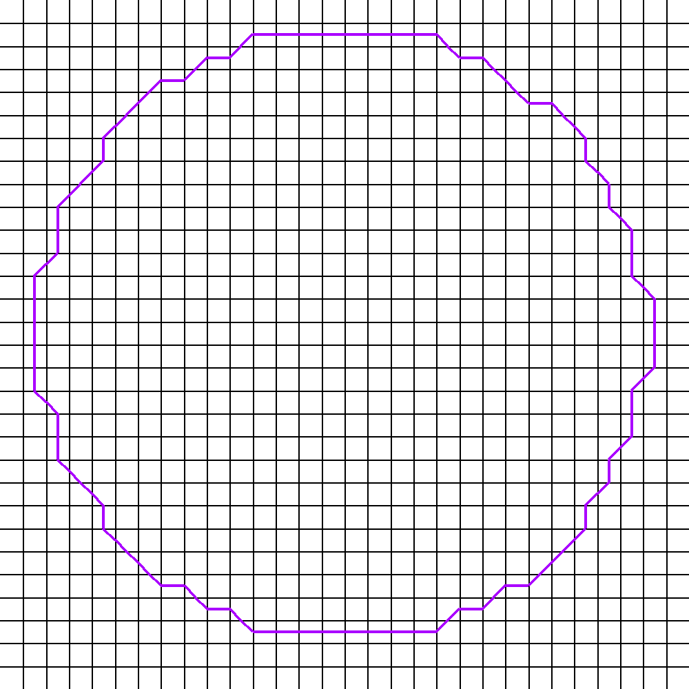
Marching Squares
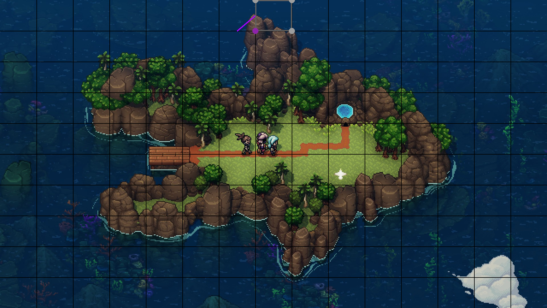
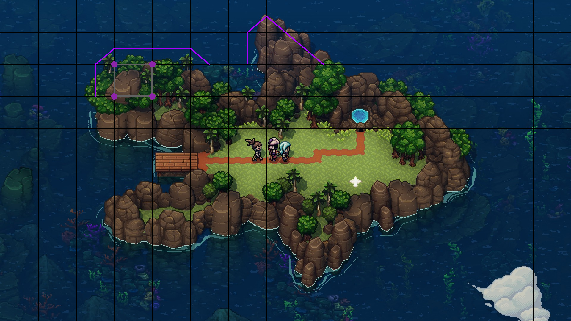
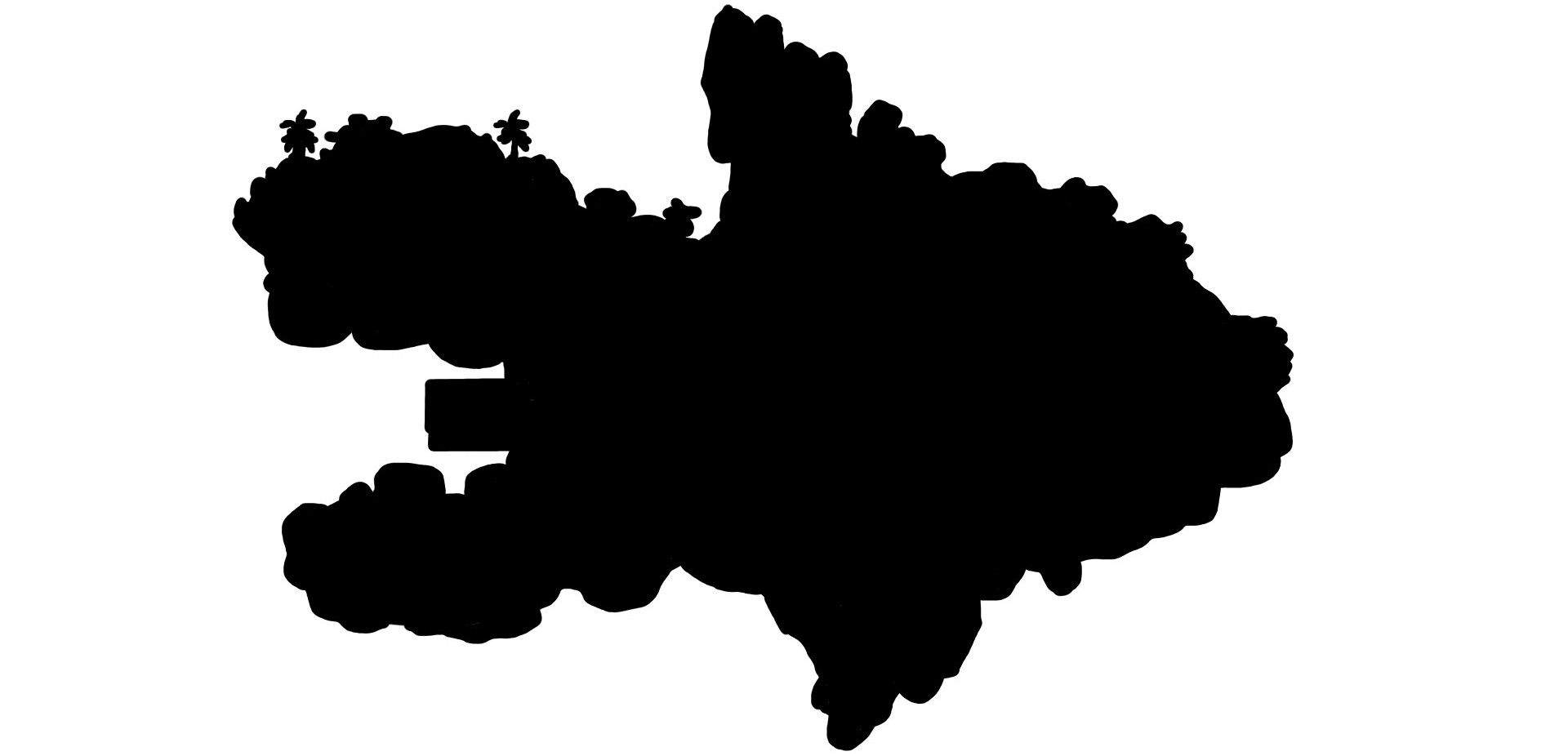
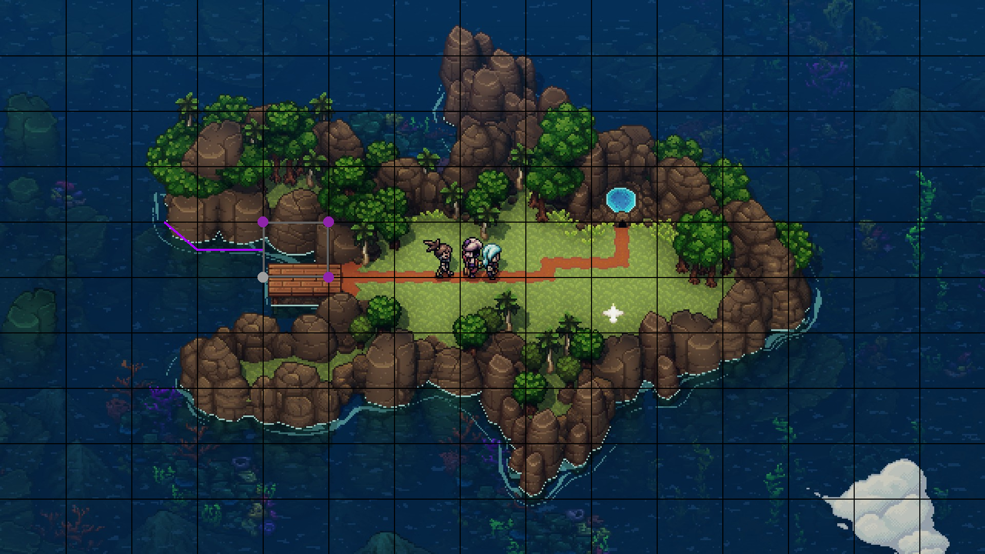
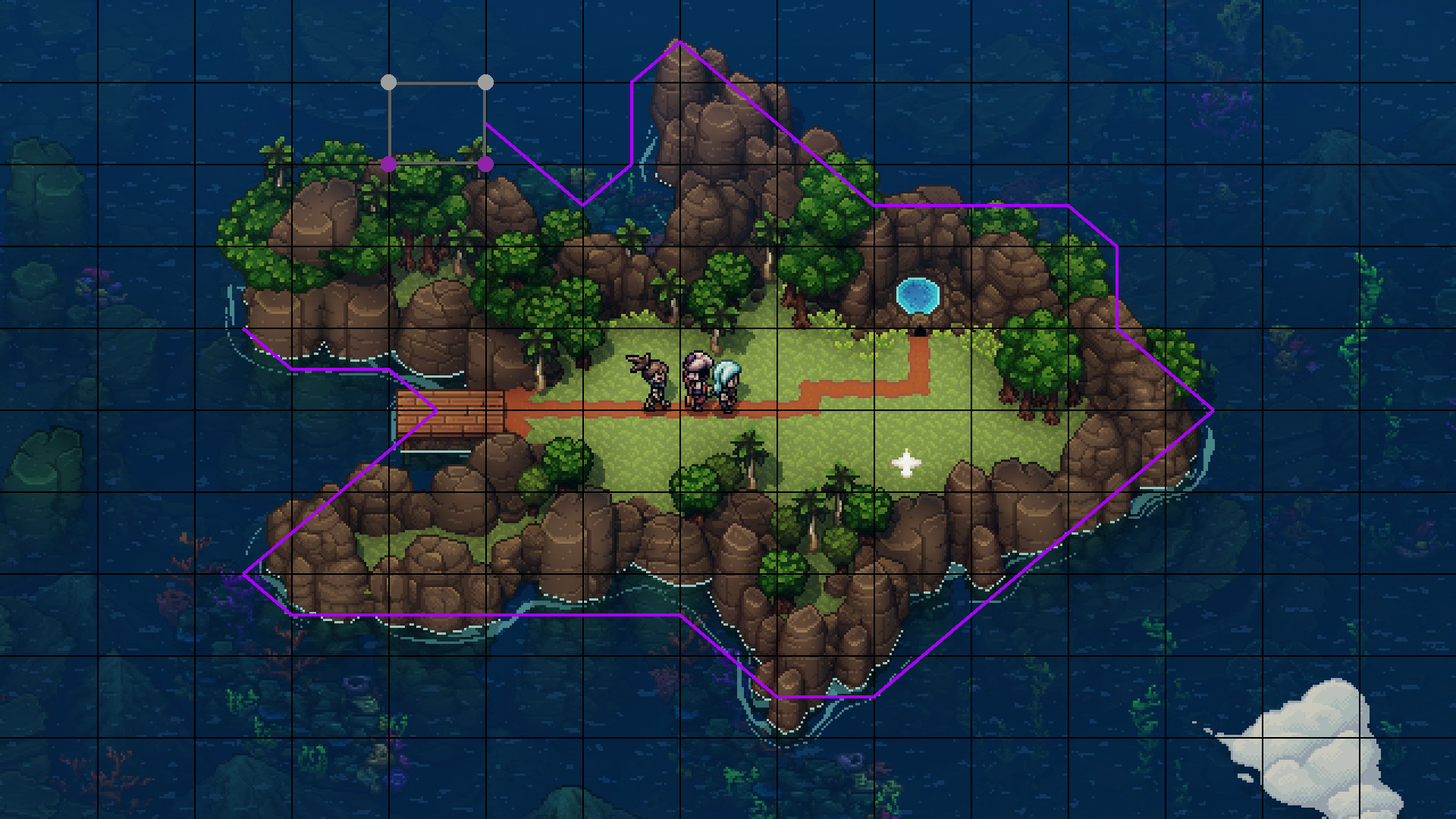
Our journey starts with an island.
© Sabotage Studio
And we need to get the
shape of the island.
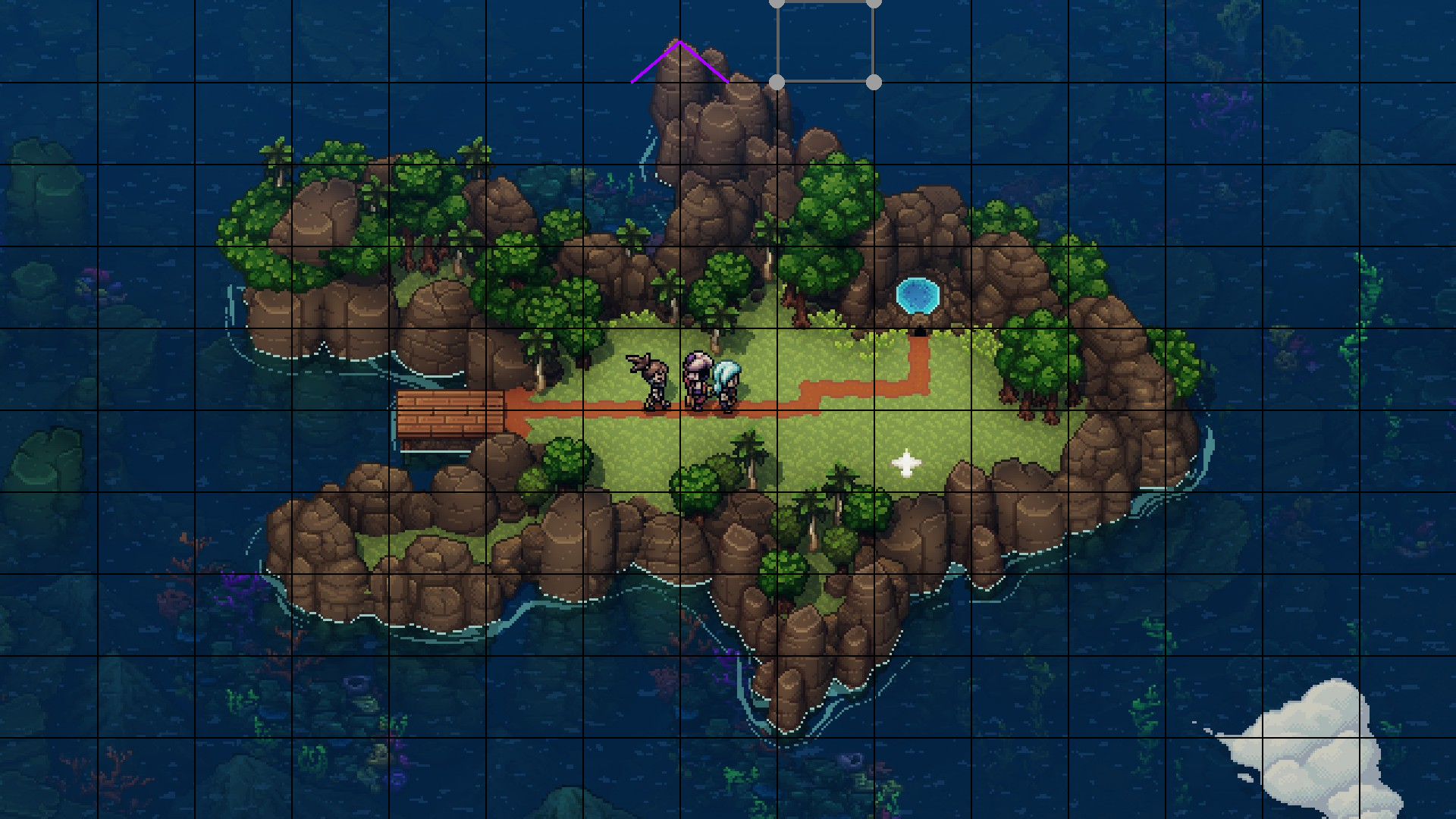
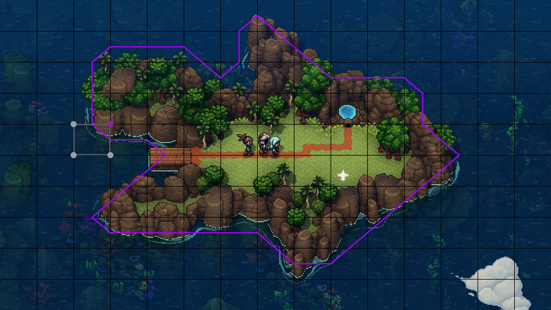
We first divide the area into a grid.
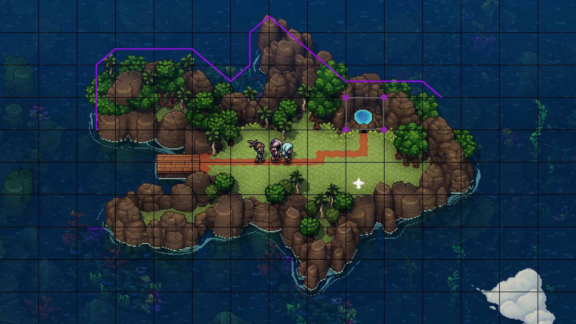
Let's inspect one cell in detail.
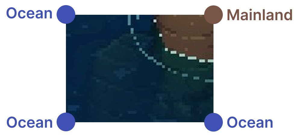
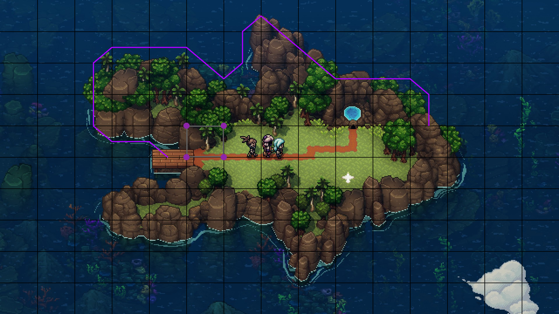
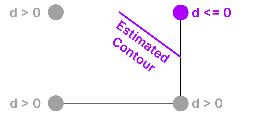
Using the corners, we can sample four points and check if they are part of the ocean or the mainland.
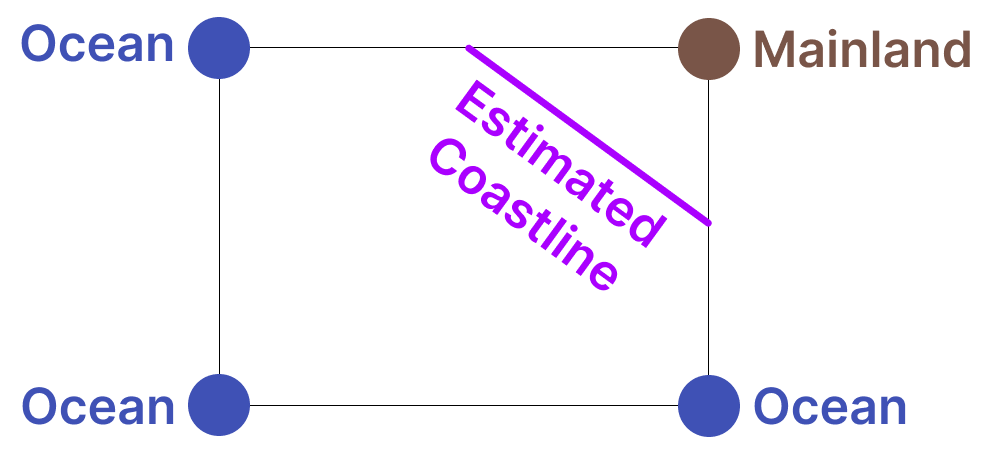
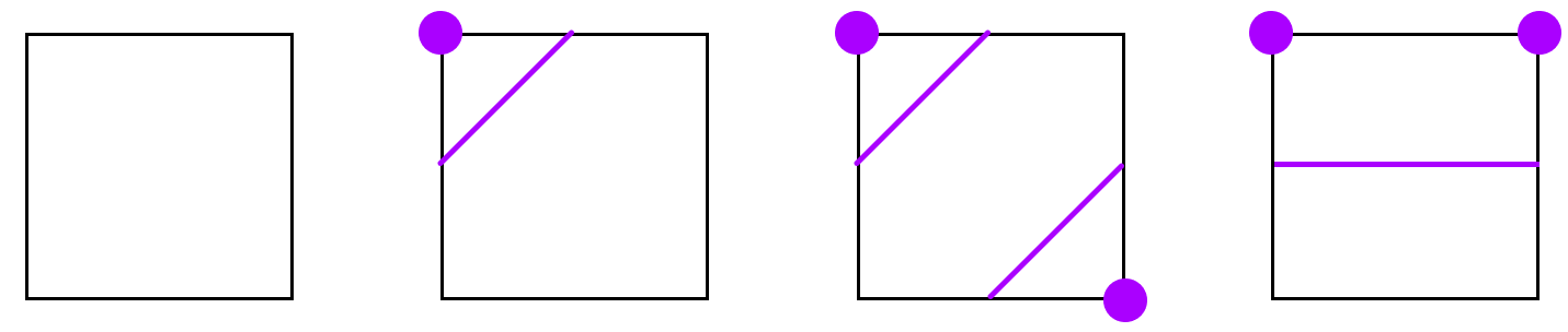
Based on the four sample points, we can estimate how the coastline might pass through the square.
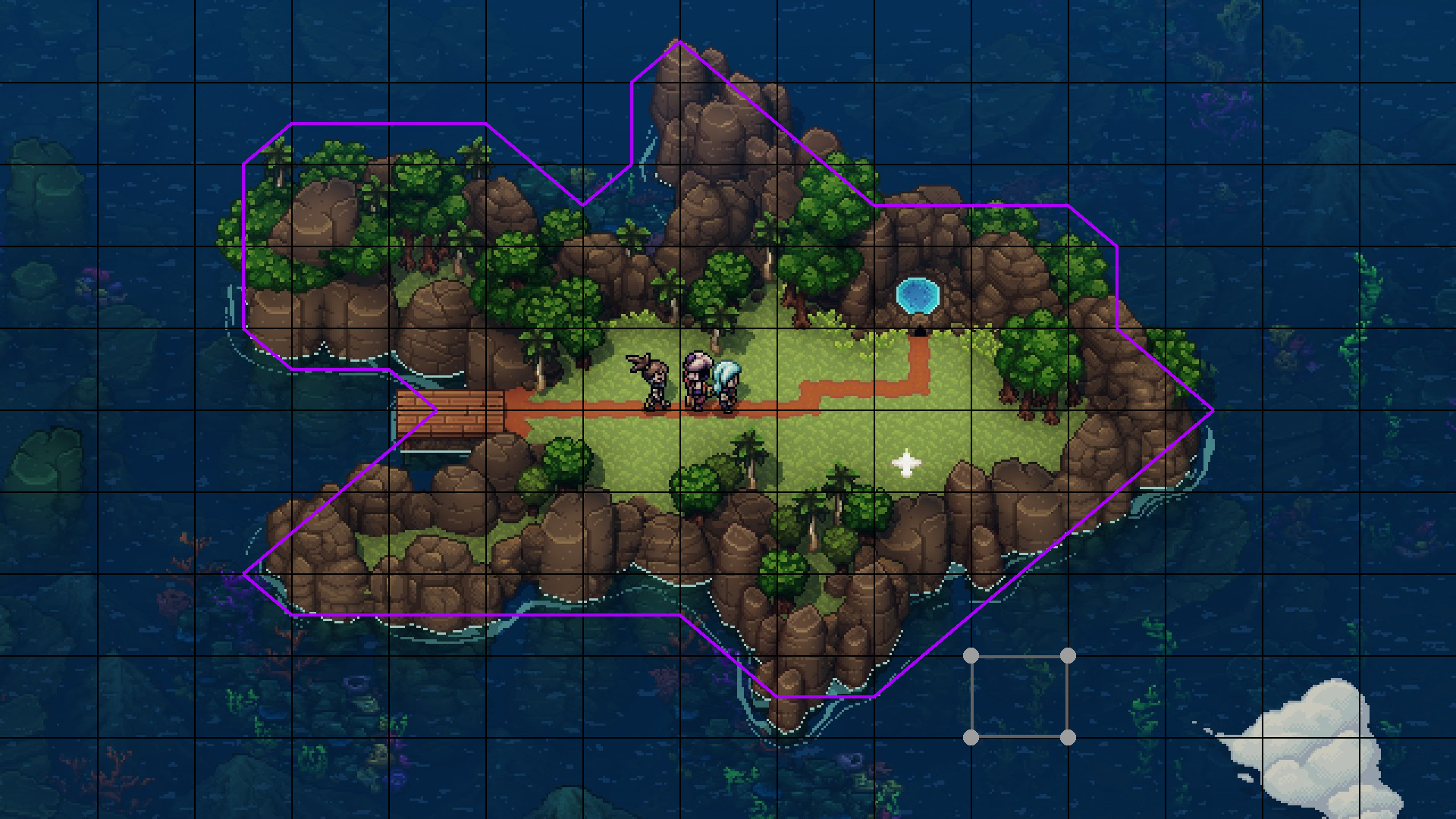
The possible number of intersections
- Each corner is binary (=2 states)
- We have four corners
- $2^4 = 16$ possible intersections.
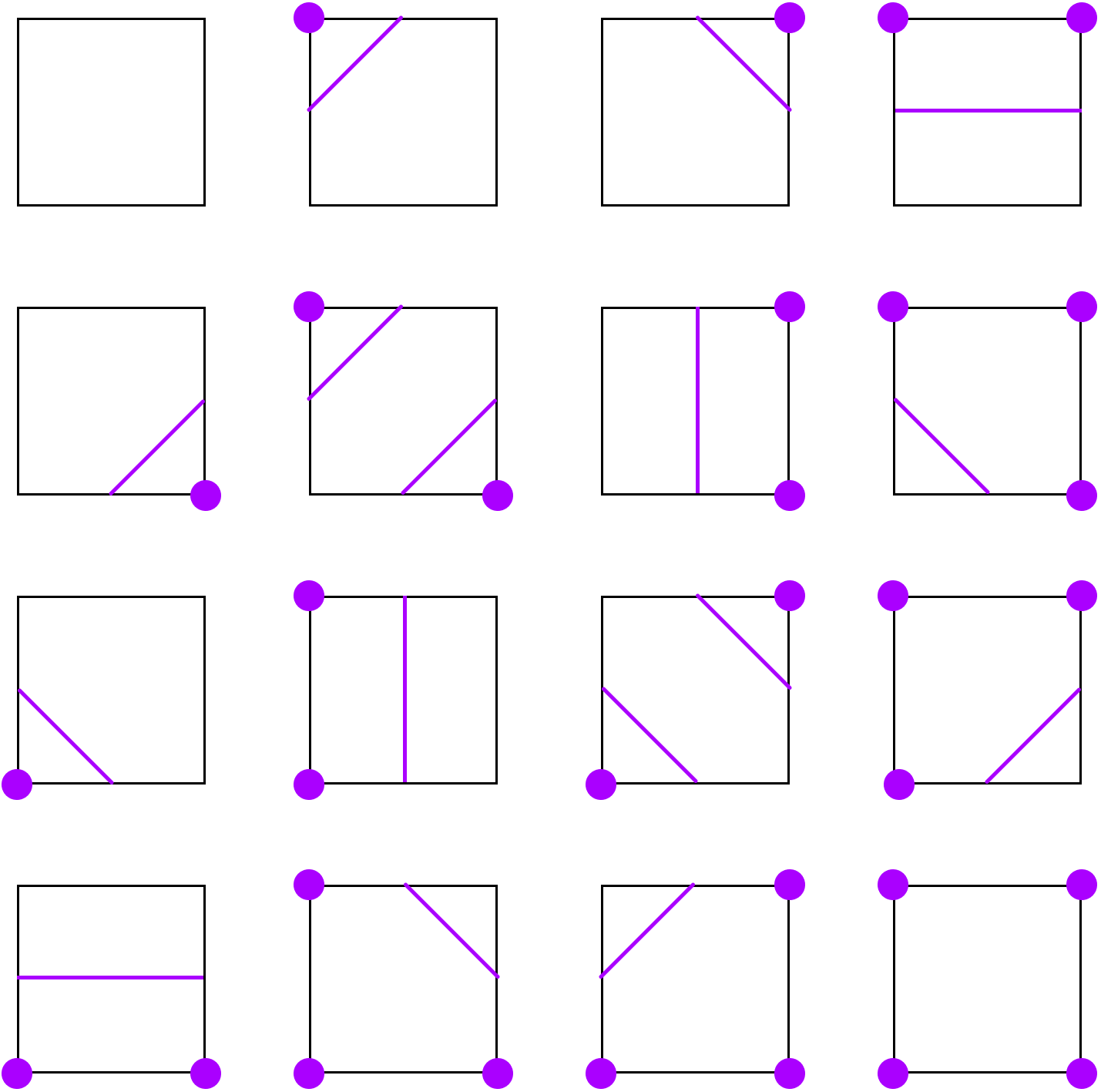
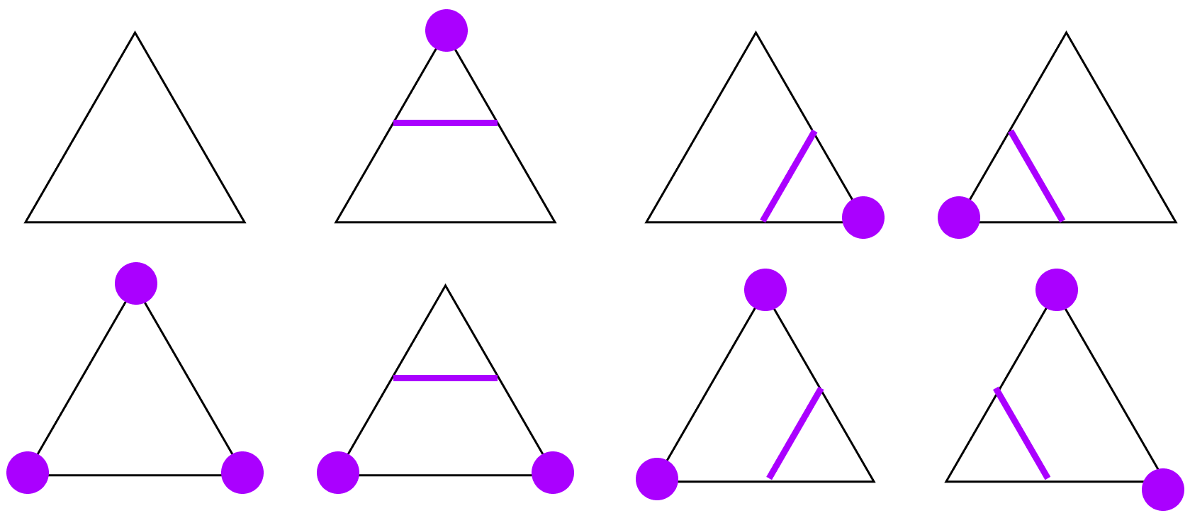
Pruning duplicates, leaves us with four patterns
- Rotational symmetry
- Mirrored symmetry
- Reflective symmetry
Now we can iterate the grid
and construct the
coastline.
Iteration 6

Iteration 7
Iteration 8
Iteration 33
Iteration 54
Iteration 65
Iteration 94

Iteration 130
Not too bad, but the
resolution is a bit low ...
Let's increase it!
Nota Bene
We have just decided inside/outside based on
binary states (ocean / mainland) in a discrete domain (pixels).
This was meant as a toy example for didactic purposes.
This is not what Marching Square / Cubes actually uses!
The input to Marching Squares are Scalar Fields!
So what is a scalar field then?
Scalar Fields
A scalar field is a function associating a single number to each point in space.
Instead of having binary values, values are now defined in $\mathbb{R}$.
Additionally, the domain is continuously defined in $\mathbb{R}^d$ instead of being discrete.
$S: \mathbb{R}^d \mapsto \mathbb{R}$
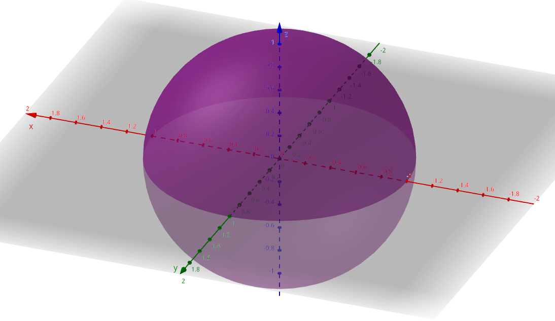
The Elliptic Paraboloid ...
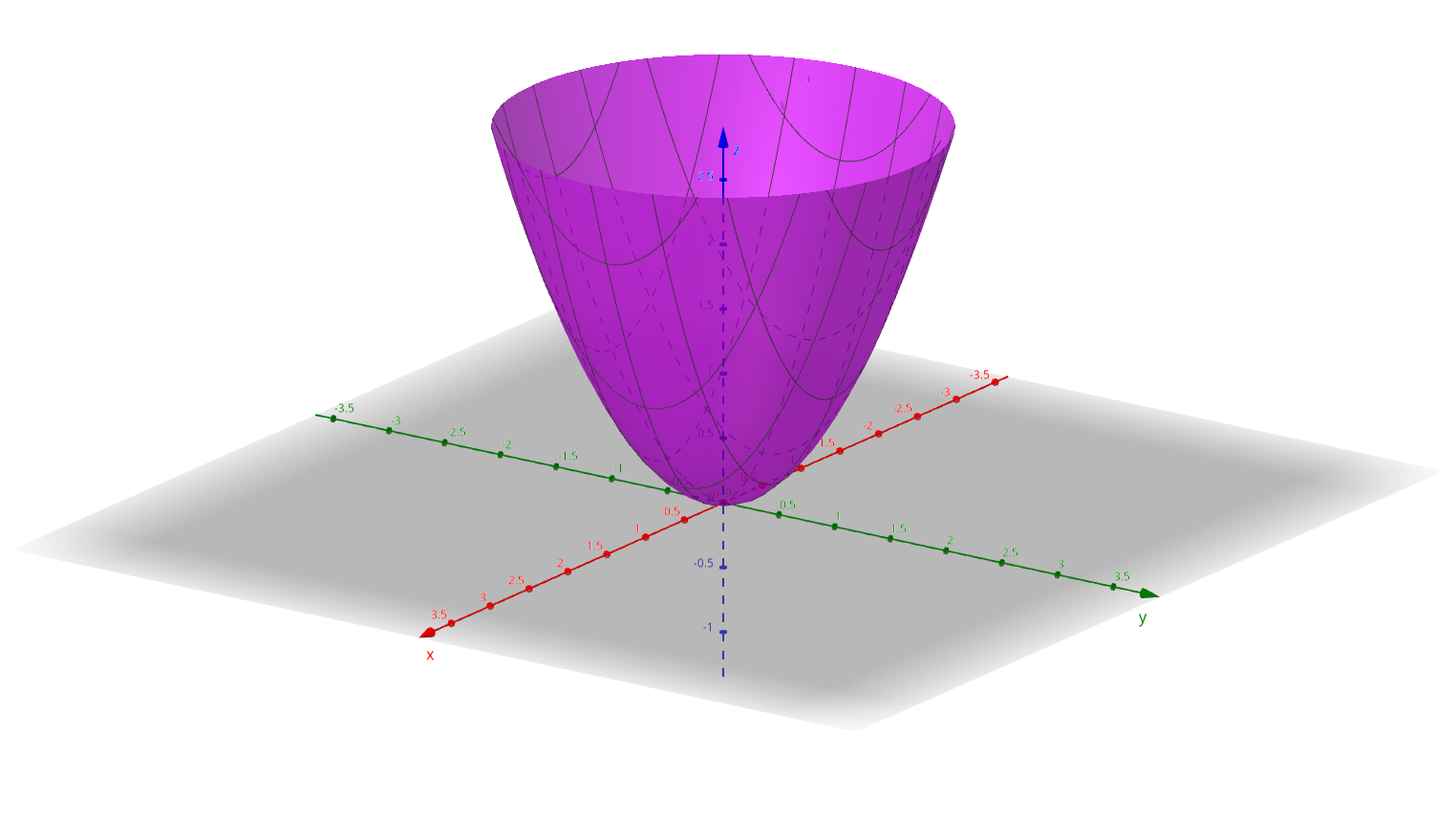
$f(x,y) = x^2 + y^2$
... has an unbounded continuous domain.
How can we extract a curve from it?
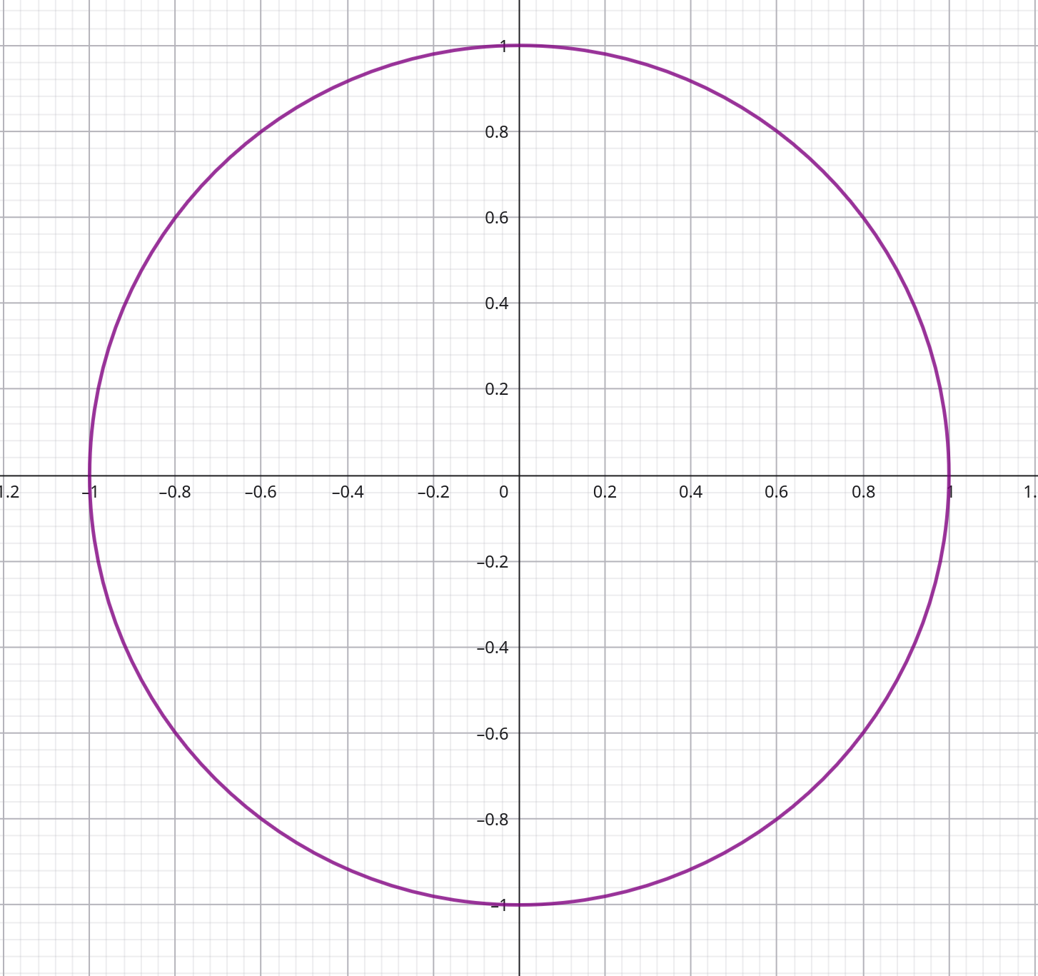
We need to define an isolevel
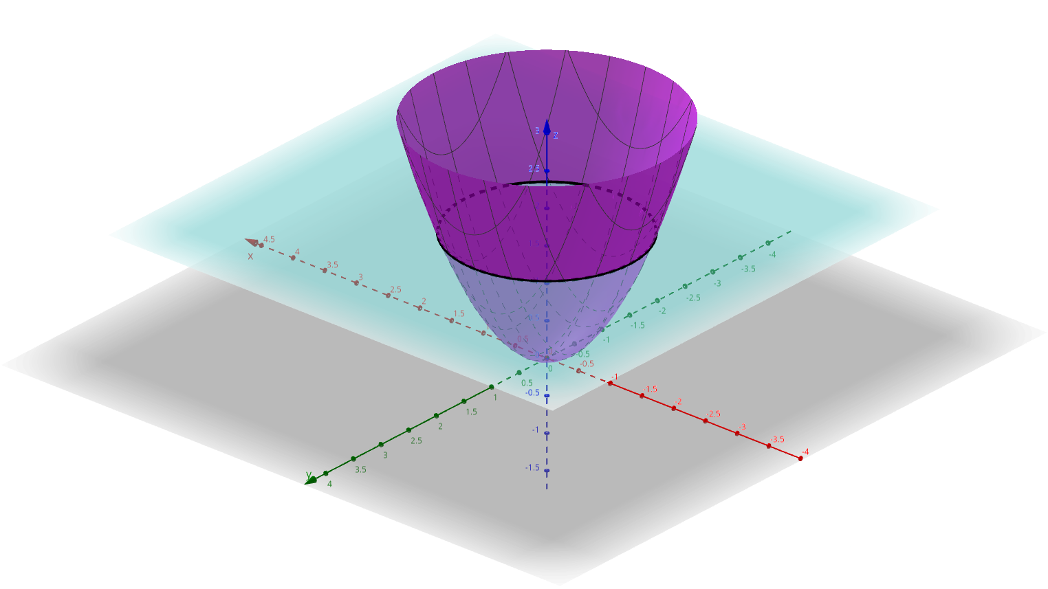
We define a plane $z = L$ where $L$ is the isolevel. The resulting interesection is given via:
$x^2 + y^2 = L$
A circle with radius $\sqrt{L}$
To create our new "mask" ...
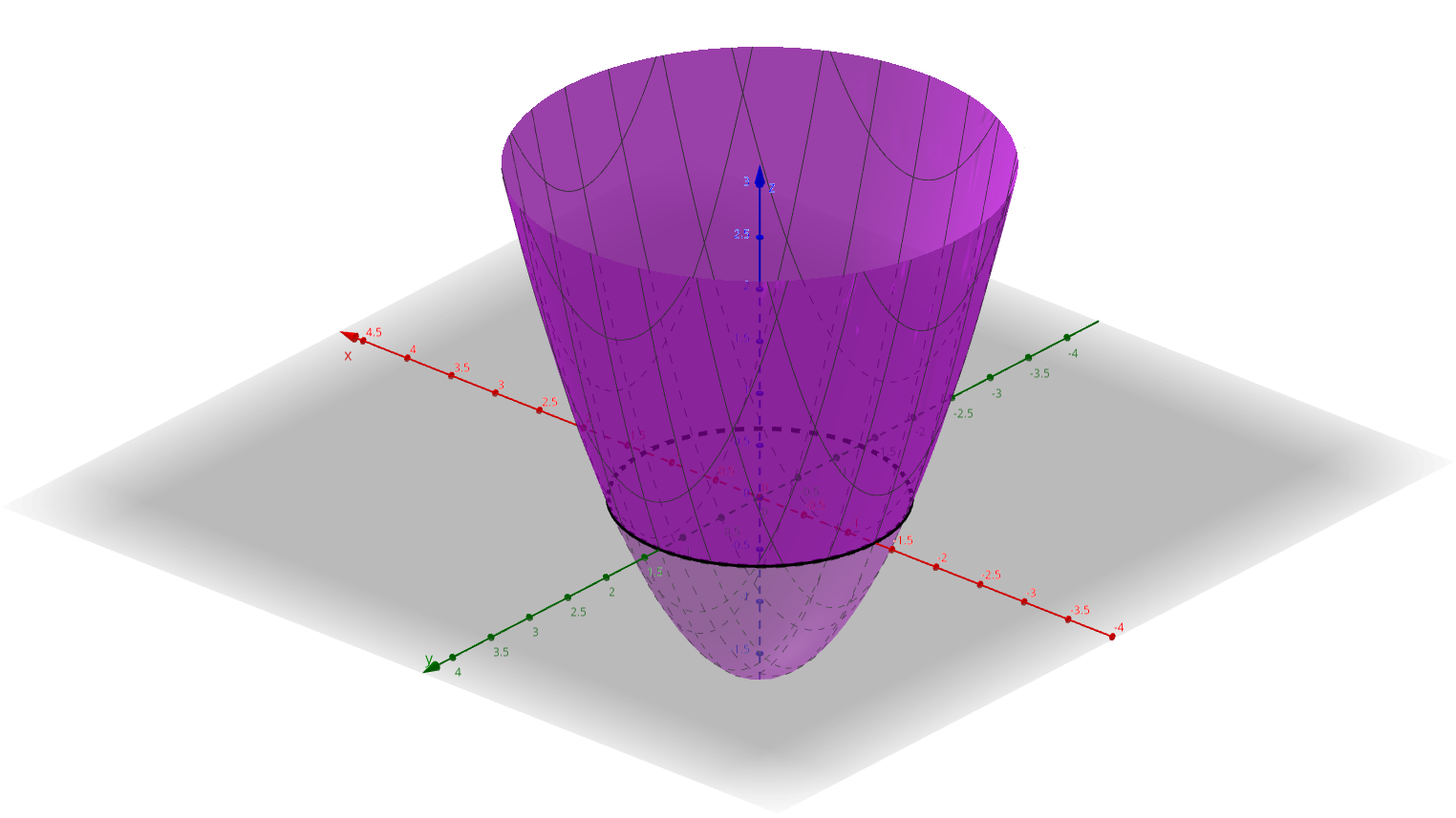
... we subtract the isolevel from the paraboloid:
$f(x, y) = x^2 + y^2 - L$
$f$ is now a Signed Distance Function (SDF)
The Signed Distance Function (SDF)
An SDF is a function, which returns the signed distance to an isolevel at any point in the domain.
$SDF: \mathbb{R}^D \mapsto \mathbb{R}$
Usually $D=2$ or $D=3$.
This means:
- Negative distance = inside the curve
- Zero distance = on the curve
- Positive distance = outside the curve
Nota bene: This assumes an isolevel of zero in the $SDF$. Choosing an isolevel of zero is a convention.
The SDF is a scalar field.
An SDF does NOT provide information about the direction!
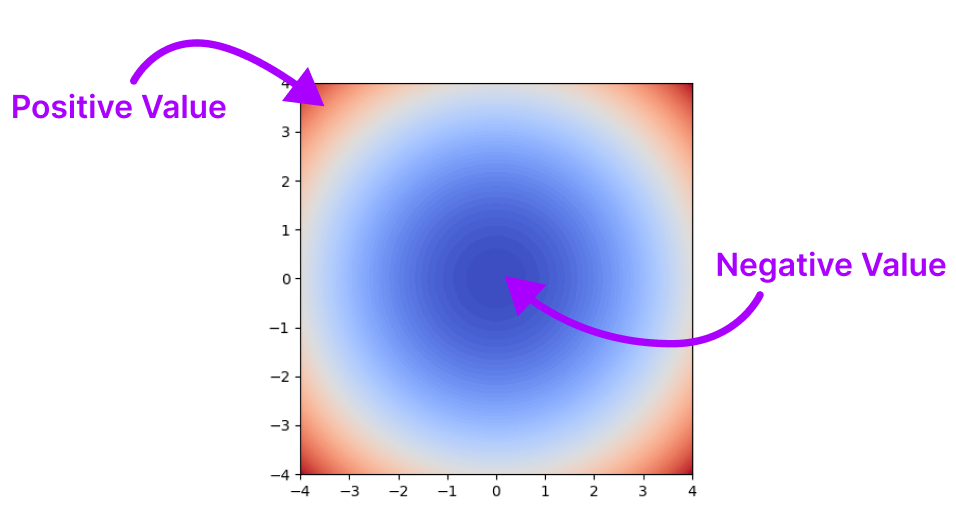
Example:

$SDF(x,y) = x^2 + y^2 - L$
Sampling from the blue zone would yield negative distance values, sampling from the red zone would yield positive distance values.
How to March Squares on an SDF (1)
Instead of having a binary sampling domain ...
... the domain is now continuous. And each corners' state is decided based on the sign of the distance value.
How to March Squares on an SDF (2)
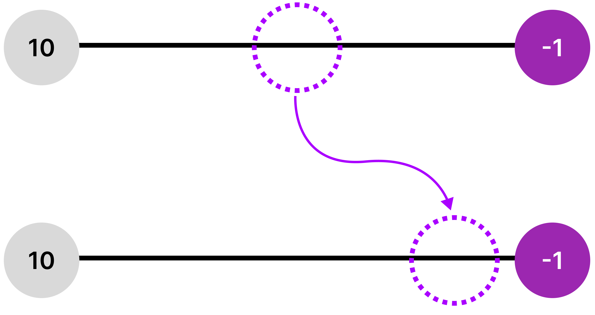
Sometimes positioning the intersection in the middle might not be optimal ...
Better: move the intersection closer to the corner that is closer to zero.
Use linear interpolation to determine position of the intersection.
The Signed Distance Field (SDFd)
Sometimes shapes like our island are hard to model as an SDF.
An SDFd is a discrete and bounded collection of scalar values.
The lookup is usually done via
indices.
$SDFd: \mathbb{I}^D \mapsto \mathbb{R}$
Where $\mathbb{I}$ is a collection of possible indices, e.g. $0$ up until the array length - 1.
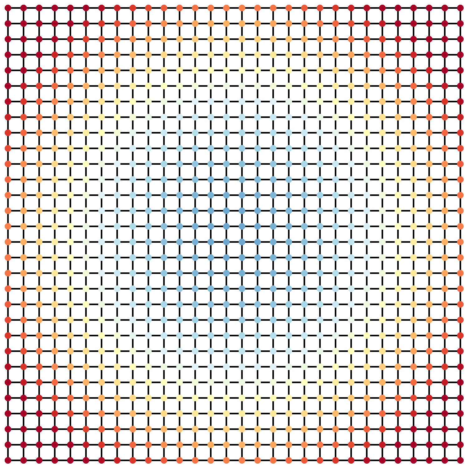
Example:
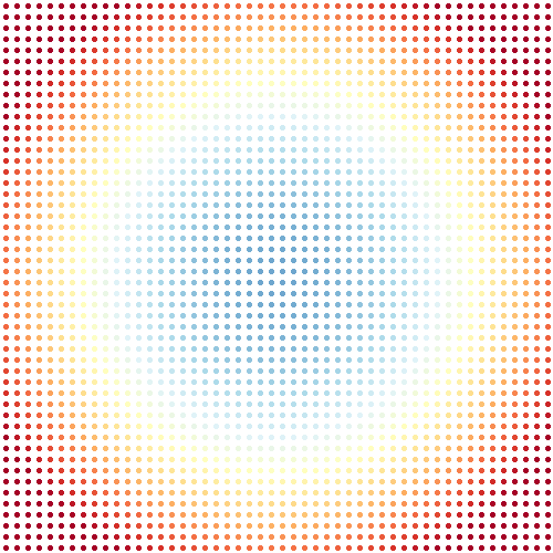
An $SDFd$ generated from our previous $SDF$.
Now we have a 50 x 50 grid of sample points instead of a continuous domain. Still, every point has a distance value!
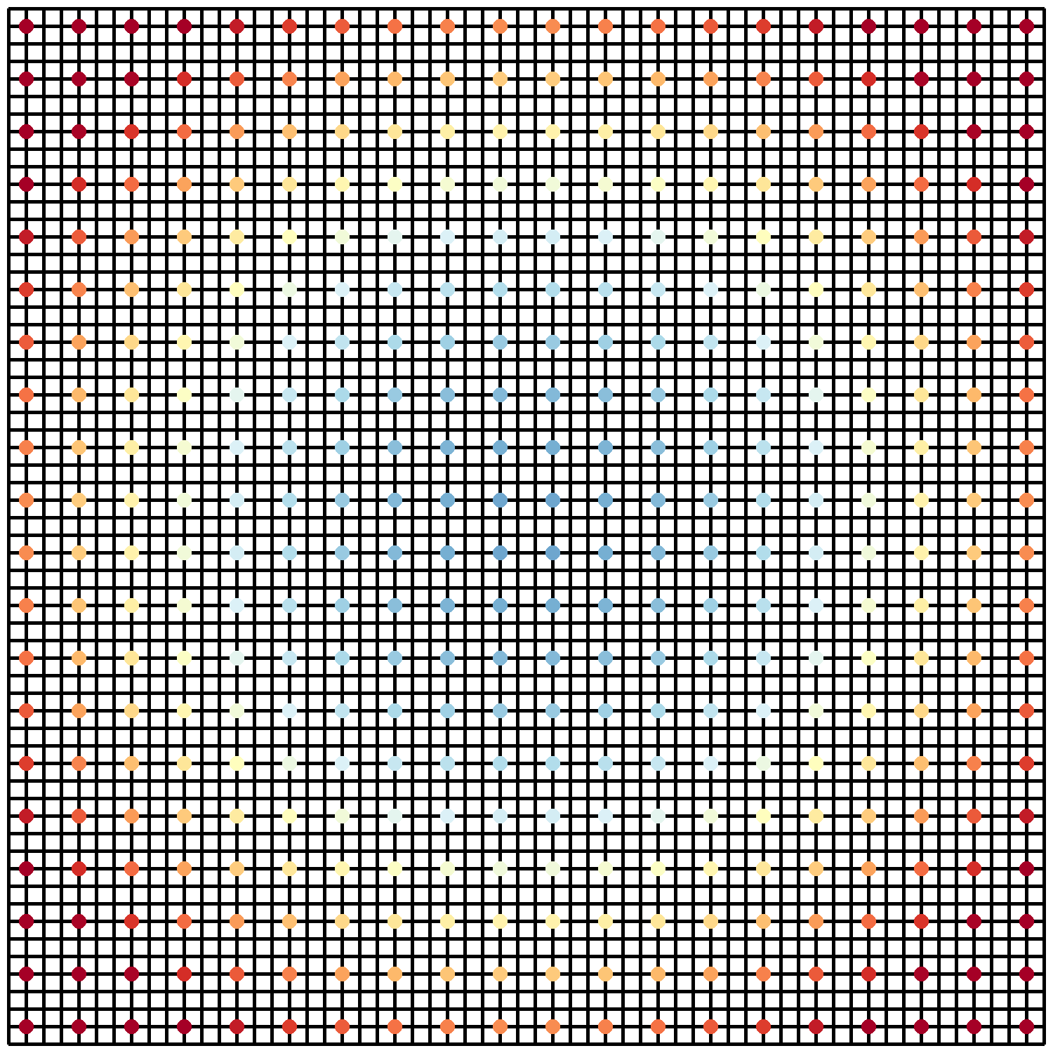
How to March Squares on an SDFd (1)

Easy Mode:
Every corner of each marching square hits exactly one value in the $SDFd$.
Procedure identical to $SDF$.
How to March Squares on an SDFd (2)
Hard Mode:
The resolution of the grid does not match the $SDFd$ resolution. Meaning: You have more corners to evaluate than you have sample points.
How to March Squares on an SDFd (3)
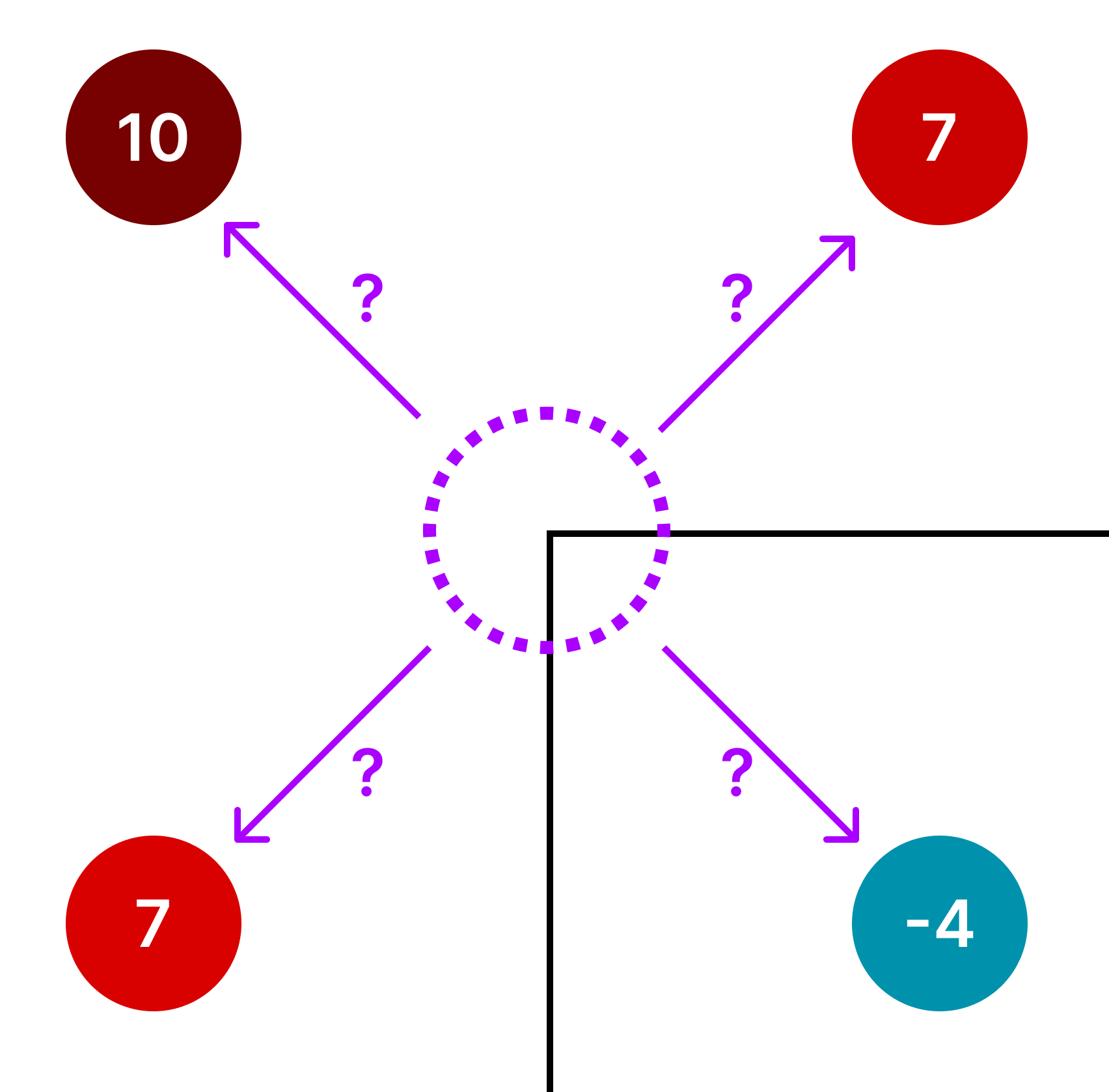
Your corner sits between four possible values.
Which distance value should you pick?
Spoiler: Taking the average of all distance values is a bit too naive.
How to March Squares on an SDFd (4)
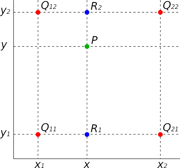
We can use bilinear interpolation.
\[ \begin{align*} R_1(x, y) &= Q_{11} \cdot \frac{x_2 - x}{x_2 - x_1} + Q_{21} \cdot \frac{x - x_1}{x_2 - x_1} \\[6pt] R_2(x, y) &= Q_{12} \cdot \frac{x_2 - x}{x_2 - x_1} + Q_{22} \cdot \frac{x - x_1}{x_2 - x_1} \\[6pt] P(x, y) &= R_1 \cdot \frac{y_2 - y}{y_2 - y_1} + R_2 \cdot \frac{y - y_1}{y_2 - y_1} \end{align*} \]All $Q$ values are distance values of the $SDFd$
$P(x, y)$ is the final interpolated distance value.
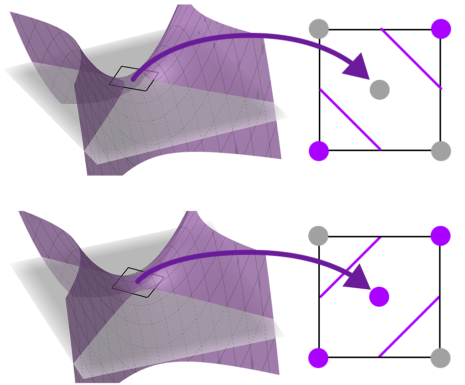
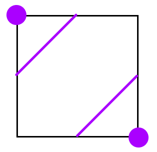
One small problem
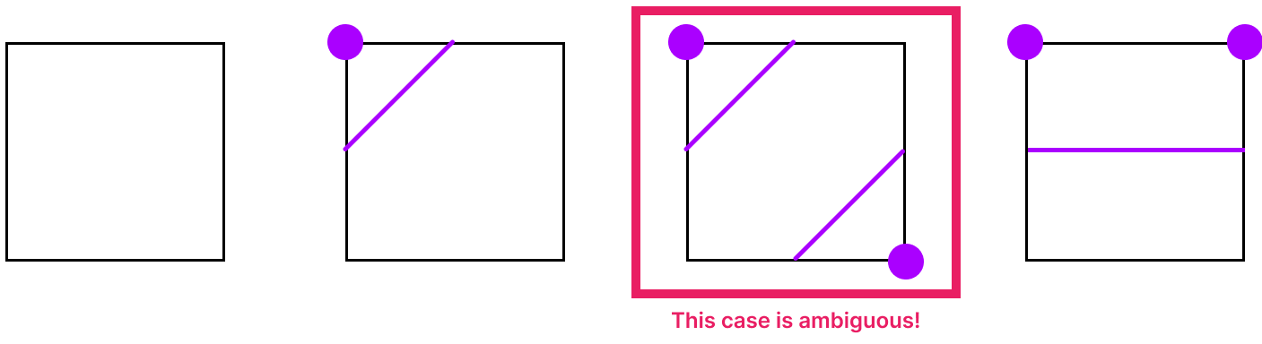
There are multiple ways to intersect this square, this is a saddle point.
We can either break the contour ...
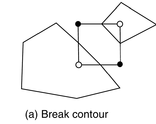
In this case the saddle point has a negative value, so it sits below the square. In this case the two contours intersecting the square belong to two different "parts".
... or join it!
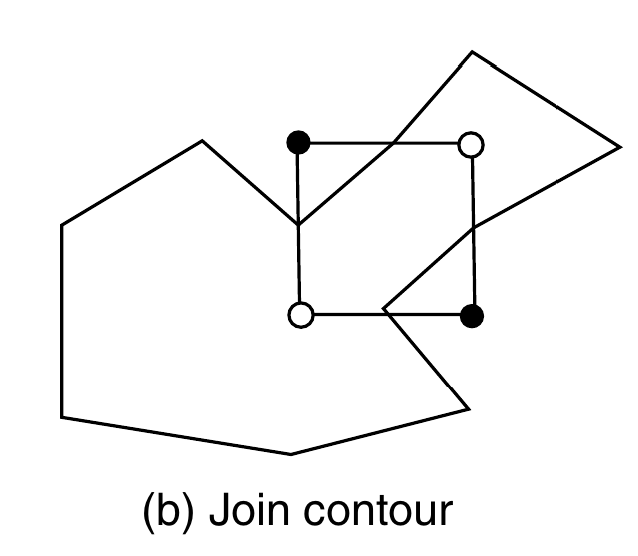
But in this case the saddle point has a positive value, so it sits above the square. In this case the two contours do not belong to two separate parts, but rather act as a "bridge".
Solution 1: Take another sample!
$\rightarrow$ Separating Polarity
By taking another sample in the center of the square, we can now eliminate the ambiguity.
$\rightarrow$ Non-Separating Polarity
Solution 1: Take another sample!
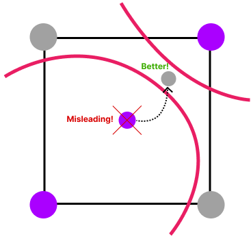
Evaluating in the geometric barycenter may be too naive!
Instead we should rather move the point towards the saddle point.
Solution 1: Take another sample!
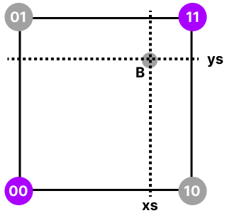
Use bilinear interpolation to determine the sample location.
$d = f_{11} - f_{10} - f_{01} + f_{00}$
$x_s = \frac{f_{01} - f_{00}}{d}$
$y_s = \frac{f_{10} - f_{00}}{d}$
$B = p_{00} + x_s (p_{10} - p_{00}) + y_s (p_{01} - p_{00})$
Then evaluate the sample at position $B$.
This idea is based on the Asymptotic Decider.
[Nielson G, Hamann B. The asymptotic decider: resolving the ambiguity in marching cubes. In: Proceedings of visualization ’91, San Diego, 1991. p. 83–91.]
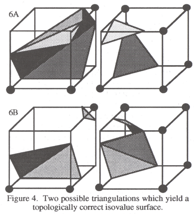
Solution 2: Marching Triangles
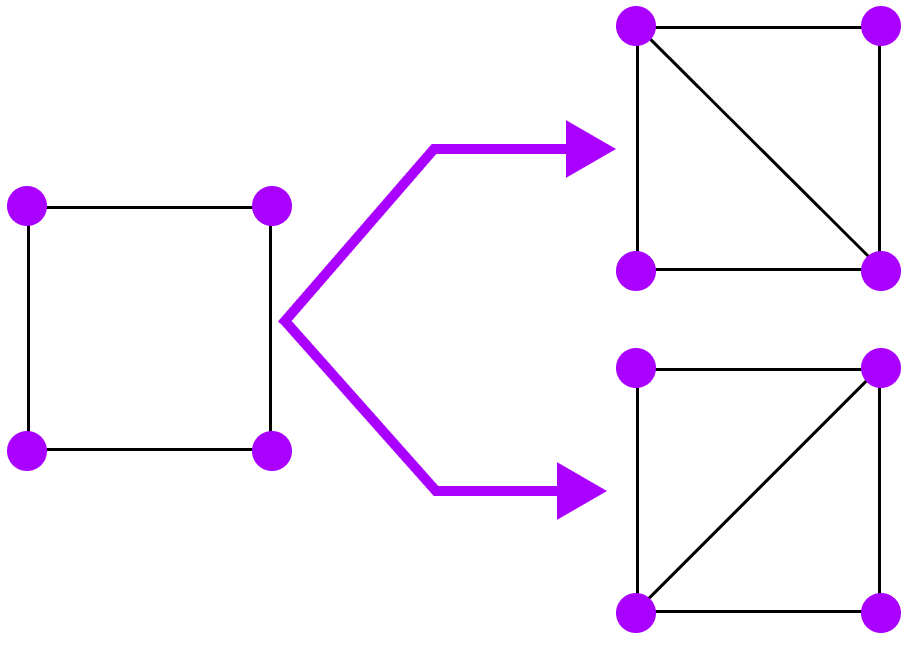
Subdivision Approach
Split each square into two triangles and compute intersections through triangles ("Marching Triangles").
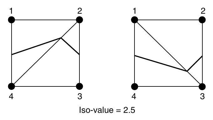
Solution 2: Marching Triangles
The case distinction is straightforward and ultimately boils down to two cases.
Most importantly: The triangles themselves do not exhibit internal ambiguity, but we now shift the global ambiguity problem to the choice of tesselation.
Minor Downside
[Johnson, Christopher R. and Charles D. Hansen. “Visualization Handbook.” (2011).]
When using marching triangles to resolve ambiguous cases on rectangular lattice, the choice of diagonal orientation can result in "bumps" in the contour surface.
"Dinosaur Back"
Warning: Terminology Collision in the Literature
Marching Triangles also refers to a surface-tracking approach.
In this lecture, we strictly mean by Marching Triangles a variant of Marching Squares shown in the previous slides.
[A.Hilton & J.Illingworth (1997). Marching Triangles: Delaunay Implicit Surface Triangulation.]
Correctness and Consistency
Correctness
Extracted contour accurately represents underlying data.
Topological Consistency
Extracted contours are continuous,
i.e. no holes.
It is possible for a contour to have a consistent topology but to not be correct.
The standard MS guarantees neither correctness nor topological consistency.
Summary of Chapter I
Marching Squares
- Divide the plane into a grid.
- Iterate all cells in the grid.
- For each cell:
- Retrieve the distance value at each corner.
- Lookup the intersection topology.
- Linearly interpolate intersections.
- Add line segment(s) to existing curve.
Signed Distance Function
Returns a distance value to the isolevel at any coordinate. $SDF: \mathbb{R}^D \mapsto \mathbb{R}$
Signed Distance Field
Returns a distance value to the isolevel at fixed indices. $SDFd: \mathbb{I}^D \mapsto \mathbb{R}$
From 2D to 3D
Marching Squares Cubes
From 2D to 3D (Inputs)
2D
Isolevels are contours / curves
$SDF: \mathbb{R}^2 \mapsto \mathbb{R}$
Bivariate Function
3D
Isolevels are surfaces
$SDF: \mathbb{R}^3 \mapsto \mathbb{R}$
Trivariate Function
From 2D to 3D (Sampling)
2D
Sampling Area: 2D Grid

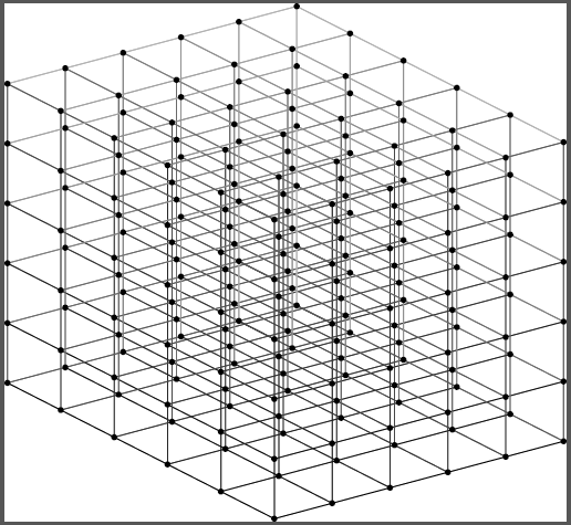
3D
Sampling Area: 3D Lattice
From 2D to 3D (Intersection)
2D
Line Segment(s)
3D
Partial Triangular Mesh
From 2D to 3D (Cases)
2D
$2^4 = 16$ cases and 4 core cases

3D
$2^8 = 256$ cases and 15 core cases
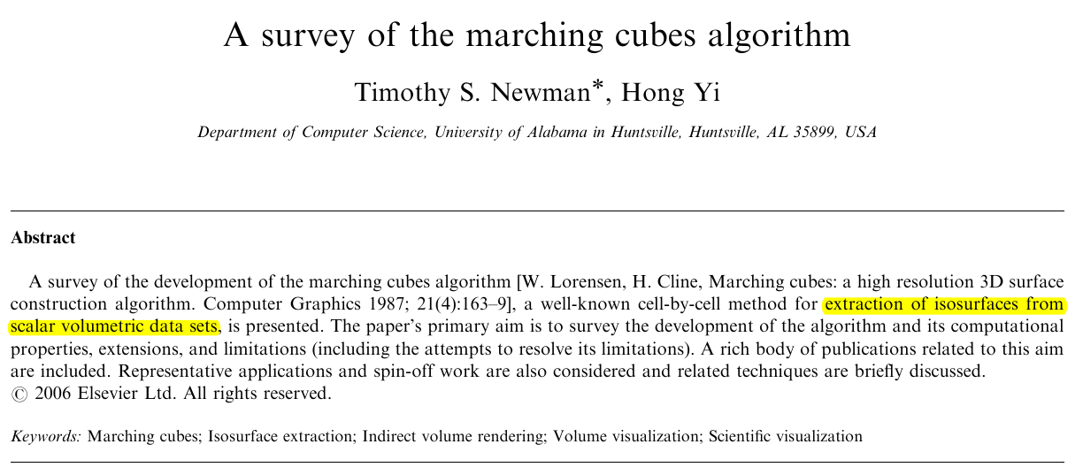
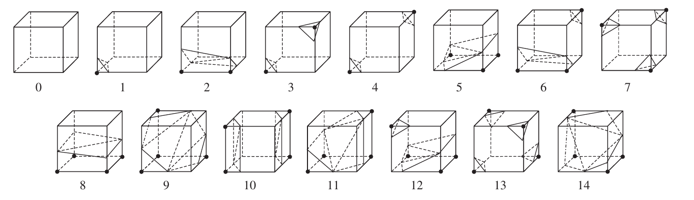 [Timothy S. Newman & Hong Yi, A survey of the marching cubes algorithm.
Computers Graphics 2006; 30:854–879.]
[Timothy S. Newman & Hong Yi, A survey of the marching cubes algorithm.
Computers Graphics 2006; 30:854–879.]
From 2D to 3D (Outputs)
2D
Output: Discrete Curve
3D
Output: Mesh
The Marching Cubes Algorithm
Marching Cubes
- Divide the space into a 3D lattice.
- Iterate all cells in the lattice.
- For each cell:
- Retrieve the distance value at each corner.
- Lookup the intersection topology.
- Linearly interpolate intersections.
- Add triangles to mesh.
[Video from live demo]
Live Demo @ fgp.tugraz.at
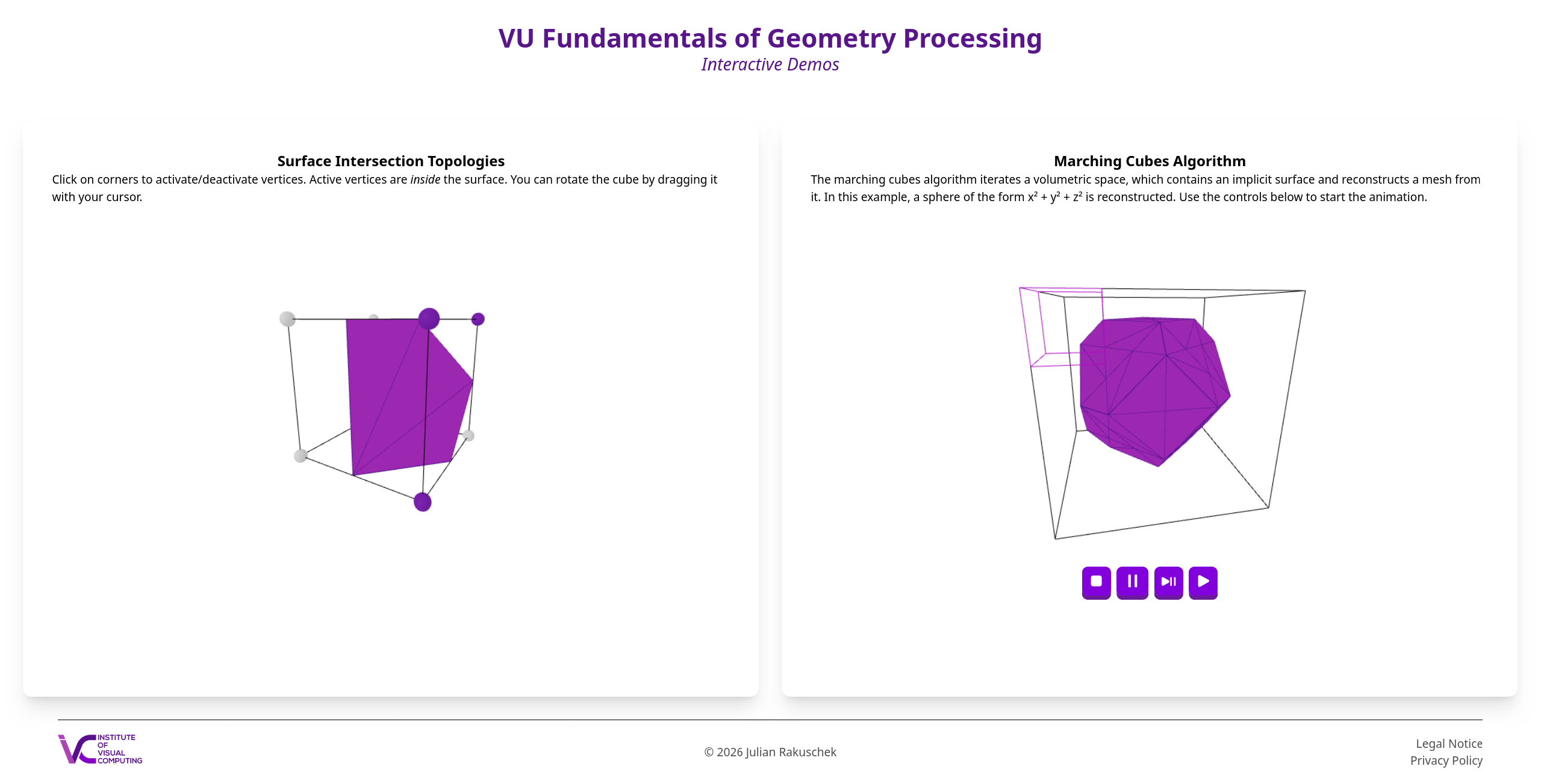
We provide a live demo where you can step through the algorithm and explore the surface intersection topologies.
LINK: fgp.tugraz.at
You will implement the Marching Cubes algorithm in A2!
Intermezzo: Assignment A2 Tutorial
This section is not relevant for the exam and is meant to provide further hints on
the assignment.
BUT: I will ask you about it in the exercise interview!
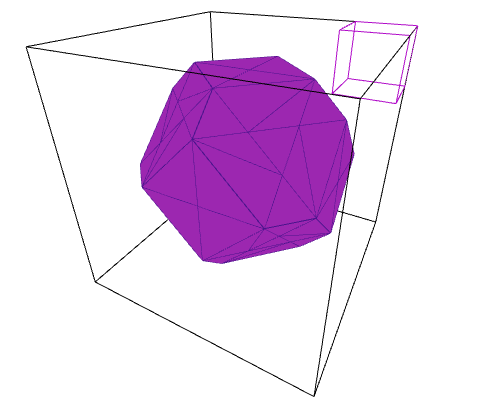
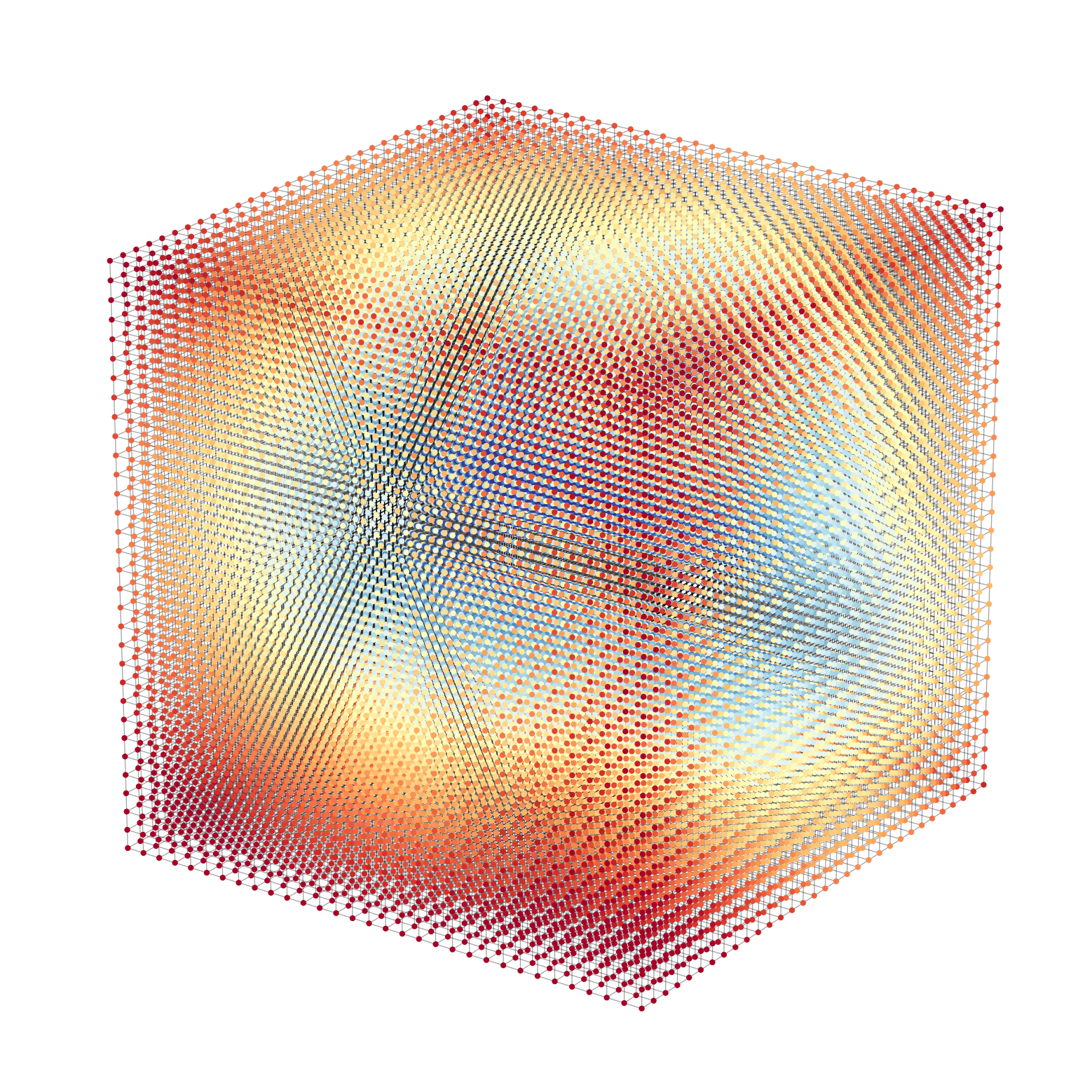
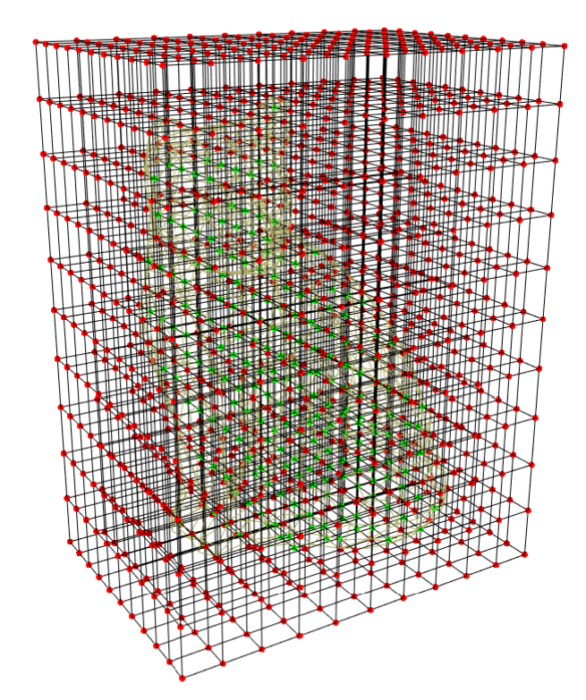
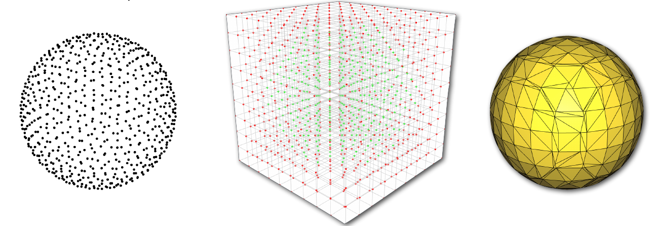
From 2D to 3D (SDFd)
Signed Distance Fields translate from a grid to a 3D lattice.
2D
3D
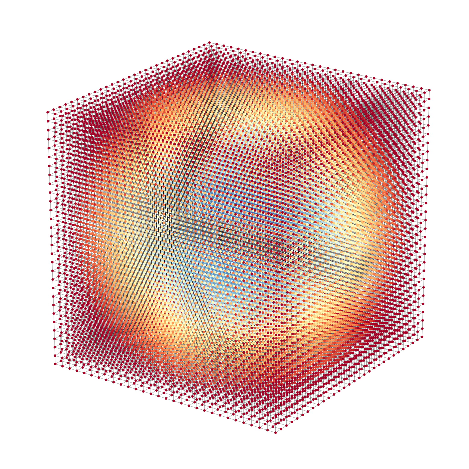
A little bit hard to see, but if you squish your eyes,
you can see the
sphere in the lattice.
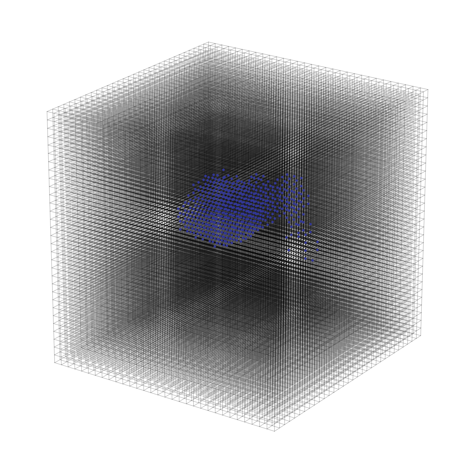
SDFd Files in the Framework
In your FGP framework, you will find *.bin files in the res/volumes folder, which are signed distance fields. These files are just flattened 3D arrays.
import numpy as np

def load_volume(filename, dimension):
    volume = np.fromfile(filename, dtype=np.float32)
    volume = volume.reshape(
        (dimension, dimension, dimension)
    )
    return volume

vol = load_volume("volume_bunny.bin", 32)
print(vol)
The framework already handles the loading for you,
but you need to retrieve the distance values.
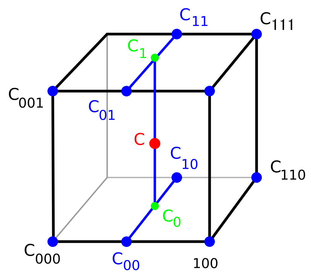
Trilinear Interpolation (1)
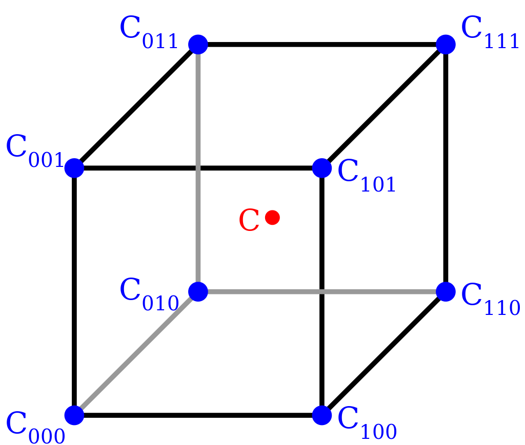
Remember: In an SDFd we only have distance values at fixed coordinates.
How can we retrieve distance values between lattice points (here at point C)? I.e. given a coordinate like (2.34123, 1.2131) how can we estimate a distance value for it?
Trilinear Interpolation (2)
In the trilinear interpolation we interpolate along every direction (first x, then y, then z).
This gives us a way to convert the SDFd to a SDF by estimating the gaps between the defined points.
All formulas are in the assignment sheet.
From Cube to Mesh (1)
We now have distance values for all eight corners.
How do we now proceed to infer the surface intersection?
From Cube to Mesh (2)
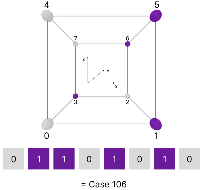
We infer the Cell Code by traversing all corners and recording the inside / outside status as a binary number.
This gives us a unique identifier for each possible surface intersection.
Use the corners array in MarchingCubes.cpp as an aid to traverse the corners in the correct order!
From Cube to Mesh (3)
With the cell code, we can retrieve the surface from the triangulation table.
Case 86 will retrieve the following triangulation[86] entry:
{
    3,0, 3,7, 2,3,
    0,1, 1,2, 6,7,
    0,1, 6,7, 4,5,
    6,7, 1,2, 2,6,
    -1,-1,-1,-1,-1,-1,-1,-1
}
Every -1 can be ignored.
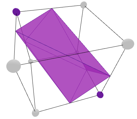
From Cube to Mesh (4)
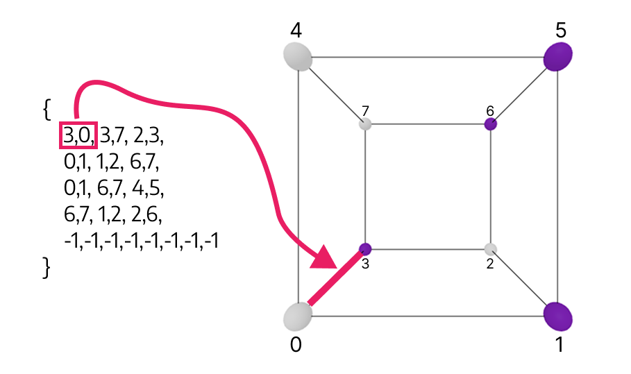
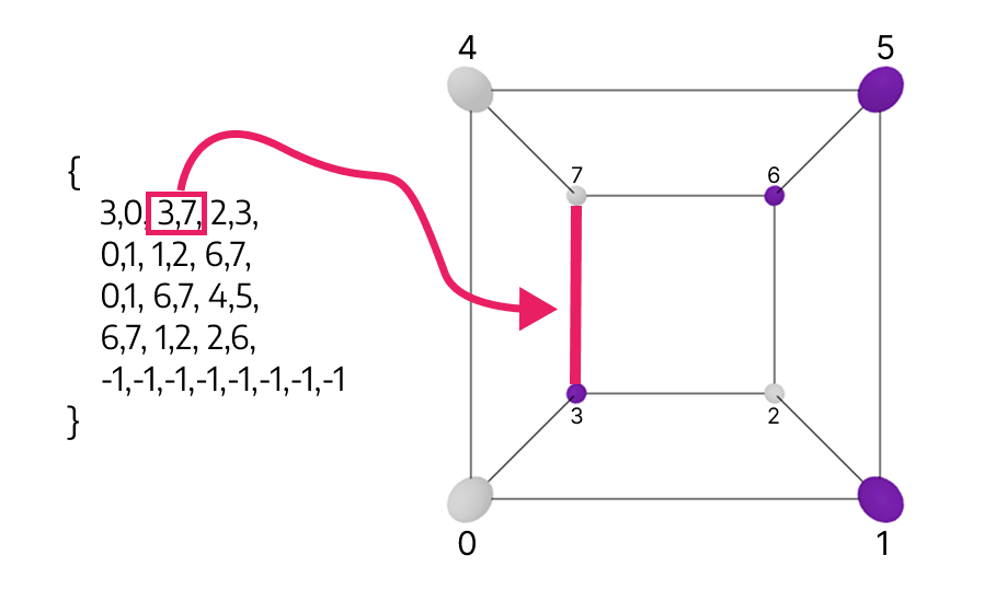
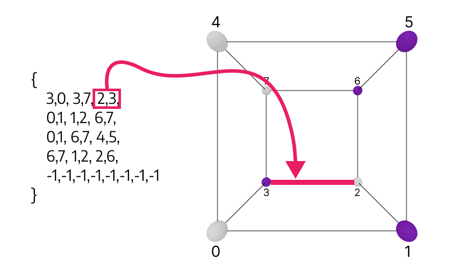
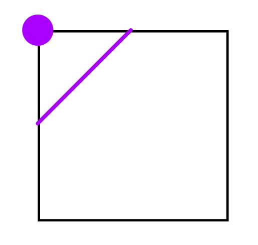
Each pair of integers represents one edge of the cube
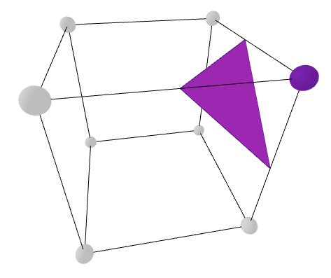
From Cube to Mesh (5)
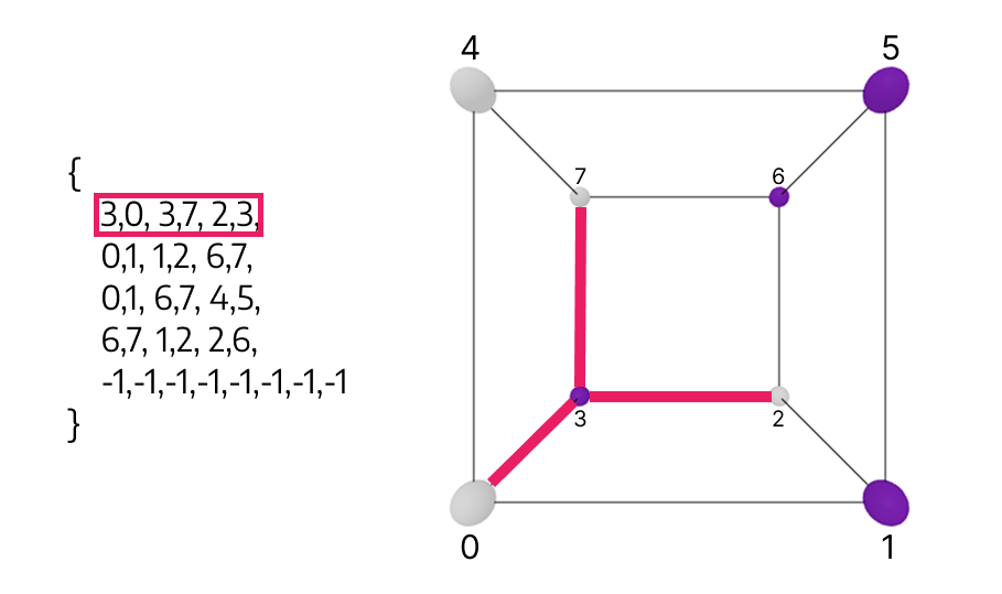
Three pairs, i.e. three edges in the cube, construct one triangle.
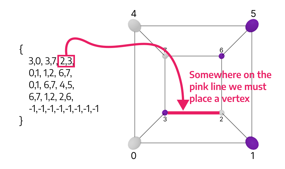
To get the corners of the triangle, we must place a vertex on each cube edge found in the triangulation table record.
From Cube to Mesh (6)
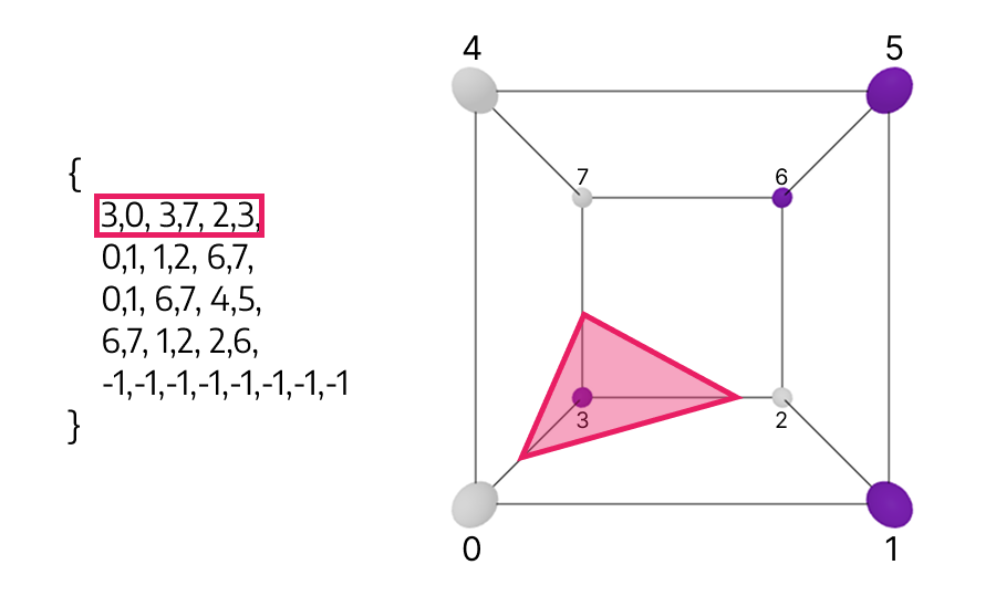
The result is a triangle that we can now add to the mesh via MarchingCubes::addTriangle.
In this assignment, you do not have to convert the triangle to the half edge data structure!
~ A2 Intermezzo End ~
Any questions on the assignment?
Note: The rest of the lecture will be relevant for the exam again!
Marching Cubes Ambiguities
Recall the ambiguity problem from marching squares
There are multiple ways to intersect this square, this is a saddle point.
Bad news: This problem persists in the 3D space as well!
Face Ambiguities (1)
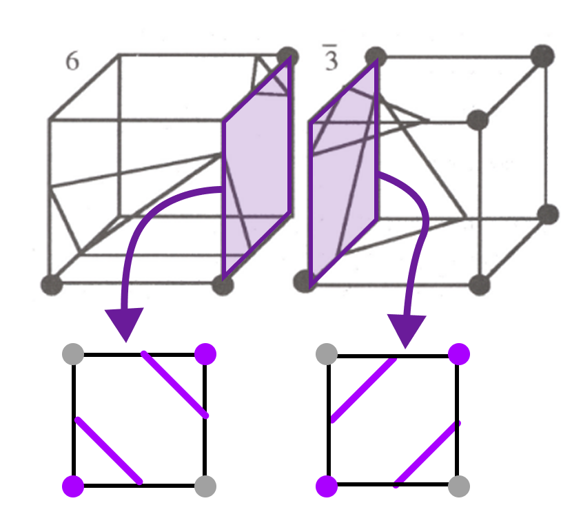
We have two neighboring cubes, naturally they share the same corner states on the shared face.
Problem: The shared face has multiple possible configurations, recall marching squares!
If the cubes are processed independently, this can result in a hole in the surface, a topological inconsistency!
$\rightarrow$ Face Ambiguity
[Nielson G, Hamann B. The asymptotic decider: resolving the ambiguity in marching cubes. In: Proceedings of visualization ’91, San Diego, 1991. p. 83–91.]
Face Ambiguities (2)
We need to make a choice: In which direction should the diagonal face? Essentially we keep one cube (left or right), choose its diagonal and compute a different surface intersection for the other cube.
[Nielson G, Hamann B. The asymptotic decider: resolving the ambiguity in marching cubes. In: Proceedings of visualization ’91, San Diego, 1991. p. 83–91.]
Face Ambiguities (3)
Solution 1:
Enforce one direction of the diagonal for every cube.
This means using a
fixed triangulation table.
Advantage: Easy
Caveat: You will get topologically consistent surfaces, but they may not be correct.
We chose this solution for the FGP assignment.
Face Ambiguities (4)
Solution 2:
Take another sample and use it to decide the direction.
Remember to also apply bilinear interpolation to find a suitable location for your additional sample! (see earlier slide on marching squares)
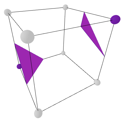
Internal Ambiguities (1)
The ambiguous case from 2D exists also in a 3D version:
2D
3D
Internal Ambiguities (2)
In 2D we could either break or join the contour:
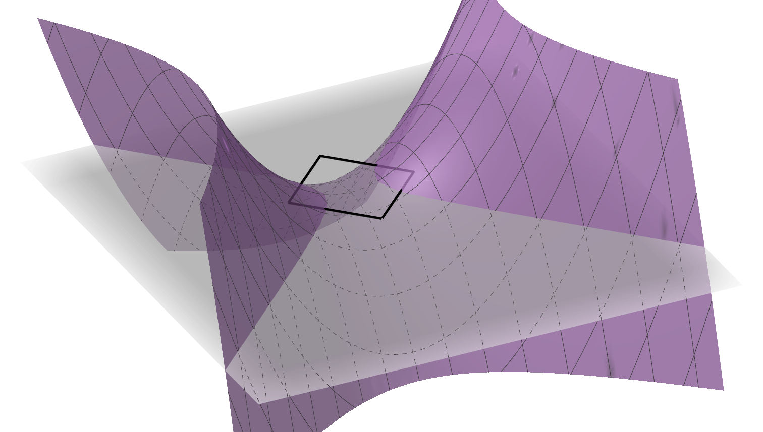
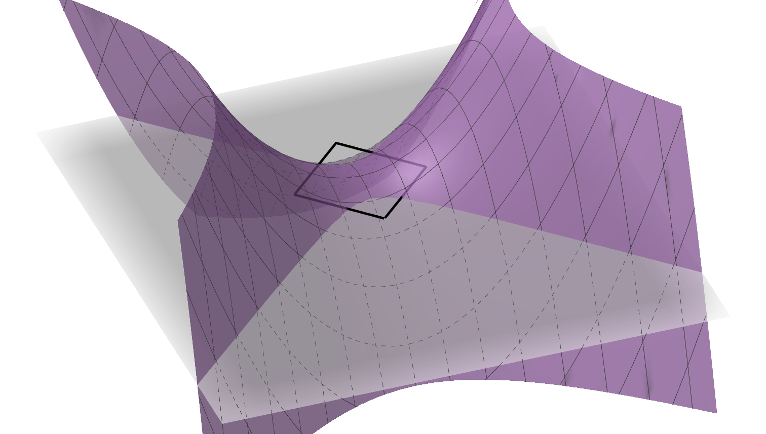
Internal Ambiguities (3)
The same "break or join" problem is now transferable to the 3D case:
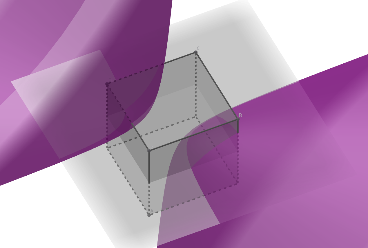
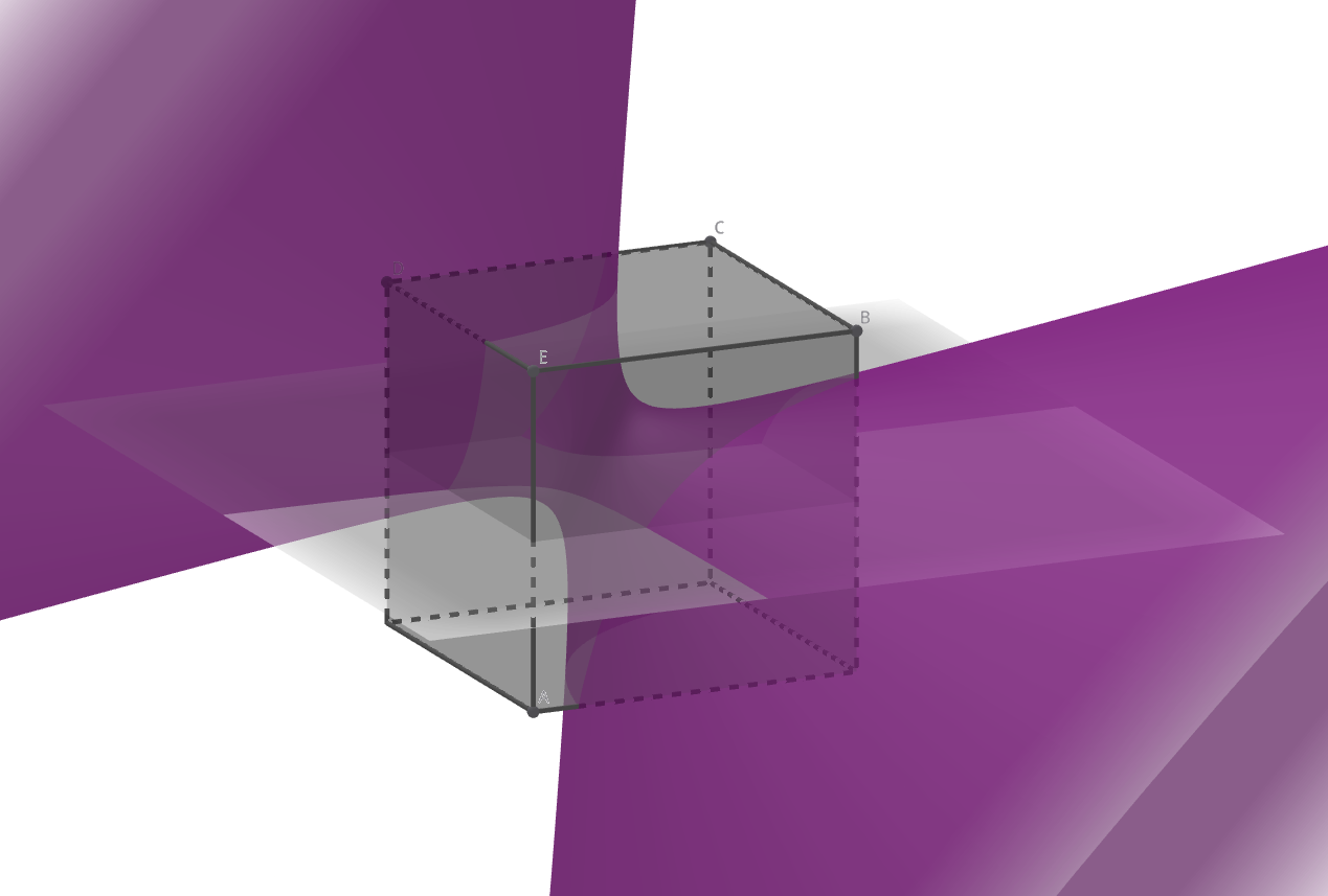
We can either break or join the hyperboloid.
Internal Ambiguities (4)
The result consists either of two separate triangles or a tube:
Internal ambiguities do not disrupt the topological consistency, but can lead to incorrect results.
Internal Ambiguities (5)
Internal ambiguity can arise in Cases 4, 6, 7, 10, 12 and 13.
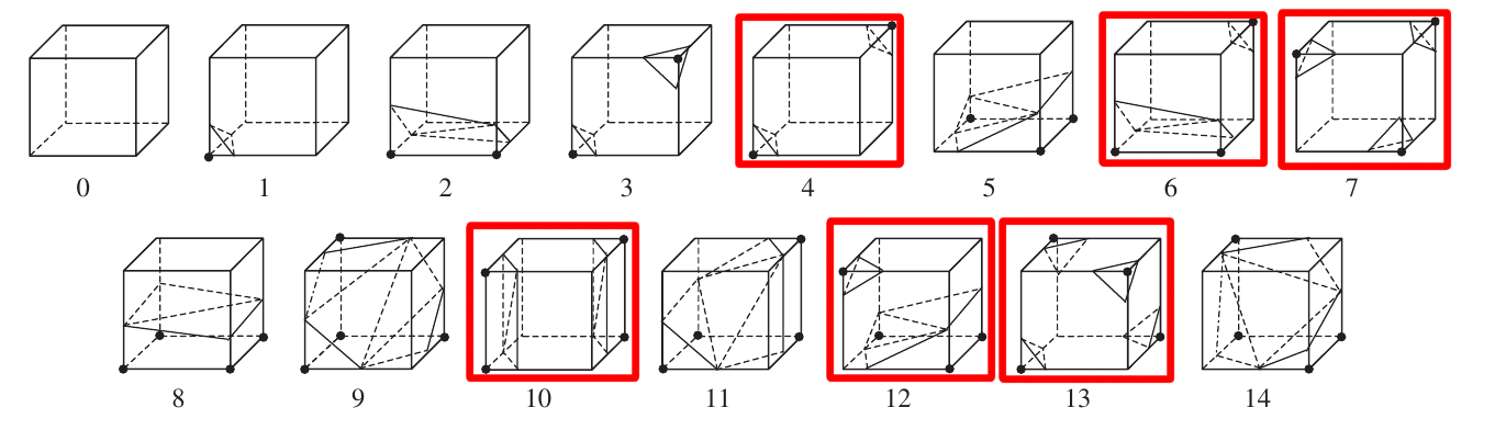
Exercise: Determine the different possible surface intersections per ambiguous case!
Can a subdivision approach help?
Marching Tetrahedra (1)
This is a tetrahedron:
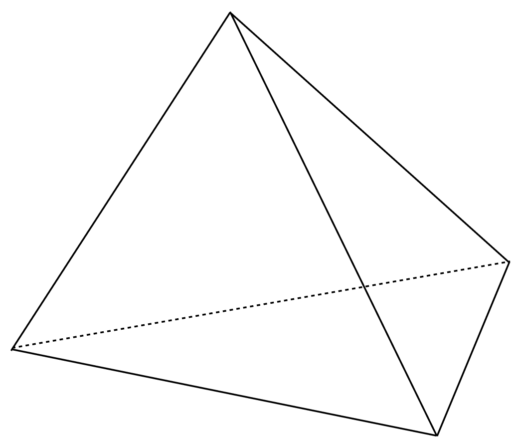
We can divide a cube into five tetrahedra:
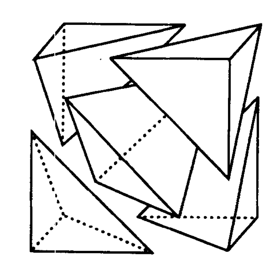
As with Marching Triangles, we can now use tetrahedrons instead of cubes.
[Zhou Y, Chen W, Tang Z. An elaborate ambiguity detection method for constructing isosurfaces within tetrahedral meshes. Computers Graphics 1995;19(3):355–64.]
Marching Tetrahedra (2)
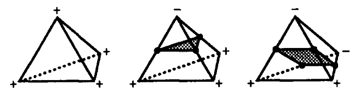
$2^4 = 16$ possible surface intersections, at the core only 3 patterns.
No internal ambiguity!
Nota bene: This does not resolve internal ambiguity of the cubes, because the problem now shifts to choosing the correct tesselation of each cube (seen in the left figure).
[Zhou Y, Chen W, Tang Z. An elaborate ambiguity detection method for constructing isosurfaces within tetrahedral meshes. Computers Graphics 1995;19(3):355–64.]
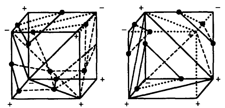
Marching Tetrahedra (3)
To connect each polygon smoothly, i.e. not to generate flaws among polygons, adjacent cubes must be subdivided in mirror-like directions.
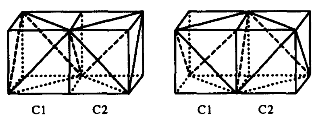
[Zhou Y, Chen W, Tang Z. An elaborate ambiguity detection method for constructing isosurfaces within tetrahedral meshes. Computers Graphics 1995;19(3):355–64.]
Several advancements can be used in MT to resolve the ambiguity problem within Cubes, but these techniques are beyond the scope of this lecture.
Further Reading:
[Timothy S. Newman & Hong Yi, A survey of the marching cubes algorithm. Computers Graphics 2006; 30:854–879.]
Do we really need to care?
One small study suggested that typically about 3%
(and
at worst 5.6%) of active cells exhibit face ambiguity.
Allen van Gelder and Jane Wilhelms. 1994. Topological considerations in isosurface generation. ACM Trans. Graph. 13, 4 (Oct. 1994), 337–375. doi:10.1145/195826.195828
Too many to ignore and too few for a serious performance overhead.
Ostrich Algorithm
- How often does the problem occur?
- How expensive is it to solve?
- Let’s do a cost-benefit analysis!
- Not worth the effort? Ignore!

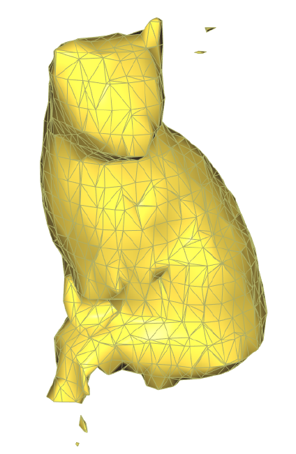
From point cloud to mesh
Geometry Acquisition Pipeline
Acknoweldgment:
This chapter is based on a lecture by Prof.in Dr.in Olga Diamanti - formerly taught in the course "Geometry for Computer Science" @ TU Graz. Her slides in turn are based on slides by Daniele Panozzo and Olga Sorkine-Hornung. The use of their figures is attributed via [Diamanti et al., 2023] to thank them for their valuable contributions.
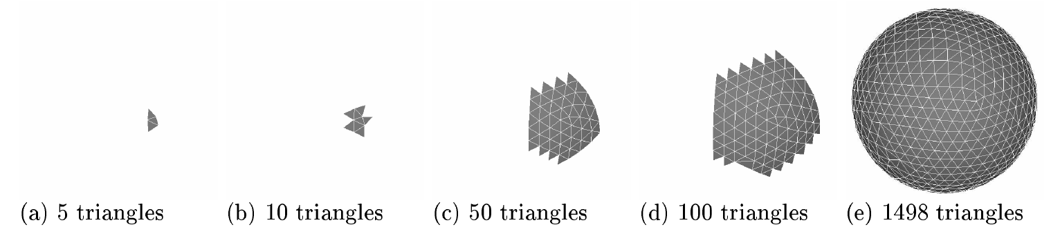
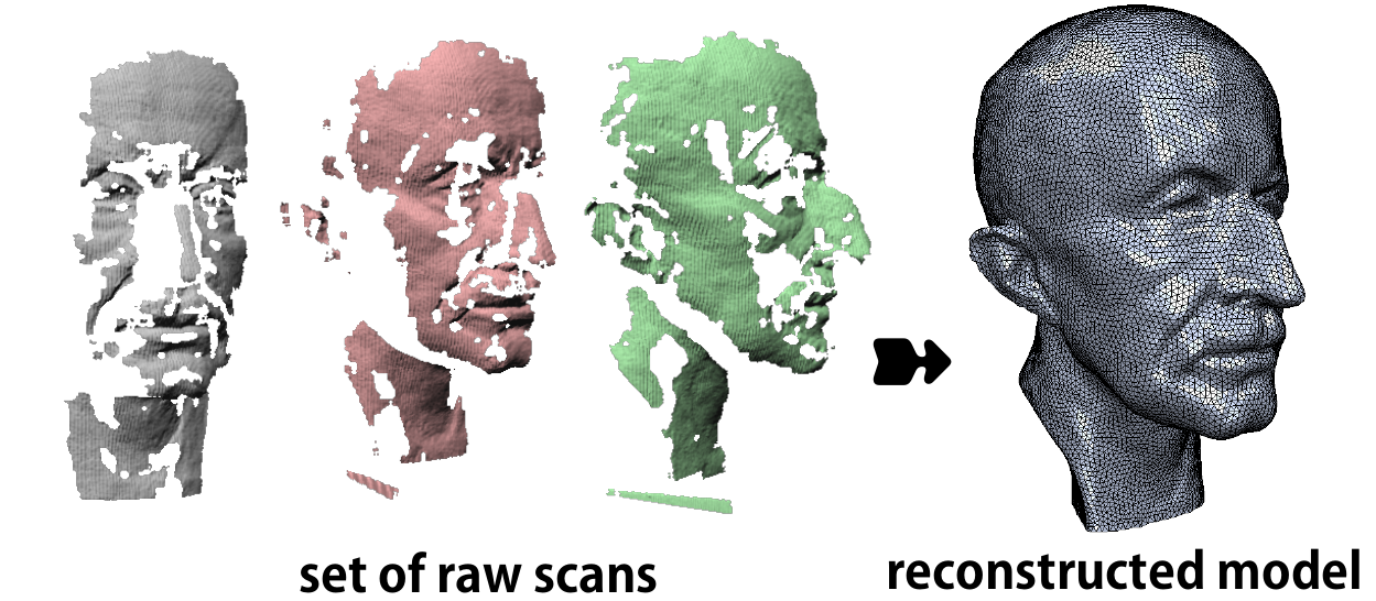
Geometry Acquisition Pipeline (1)
Scanning
We acquire points from range scanners
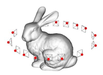
Registration
Bring all range images to one coordinate system
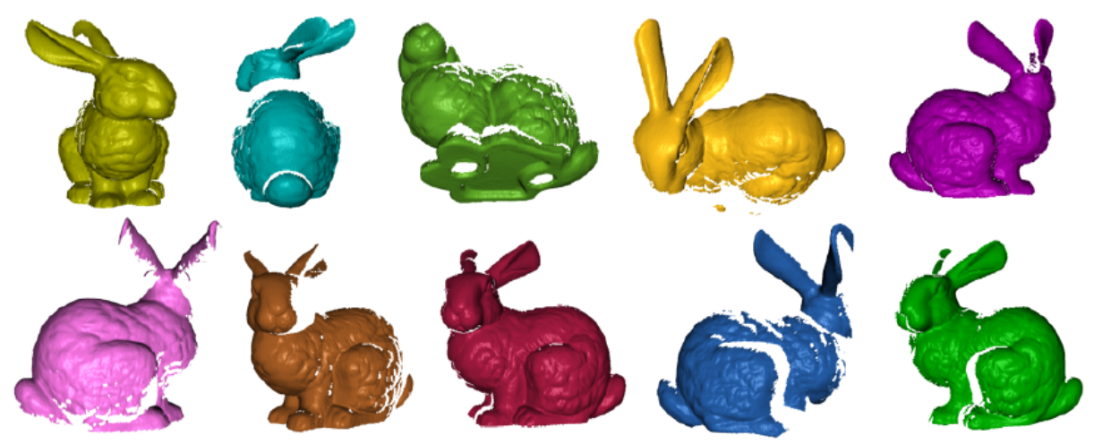
Reconstruction
Integrate scans in a single mesh
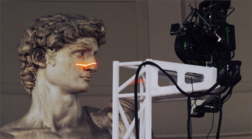
You scan an object multiple times from different sides.
Geometry Acquisition Pipeline (2)
Scanning
We acquire points from range scanners
Registration
Bring all range images to one coordinate system
Reconstruction
Integrate scans in a single mesh
[Diamanti et al., 2023]
Geometry Acquisition Pipeline (3)
Scanning
We acquire points from range scanners
Registration
Bring all range images to one coordinate system
Reconstruction
Integrate scans in a single mesh
[Diamanti et al., 2023]
Geometry Acquisition Pipeline (4)
The overall goal: Generate mesh from set of surface samples
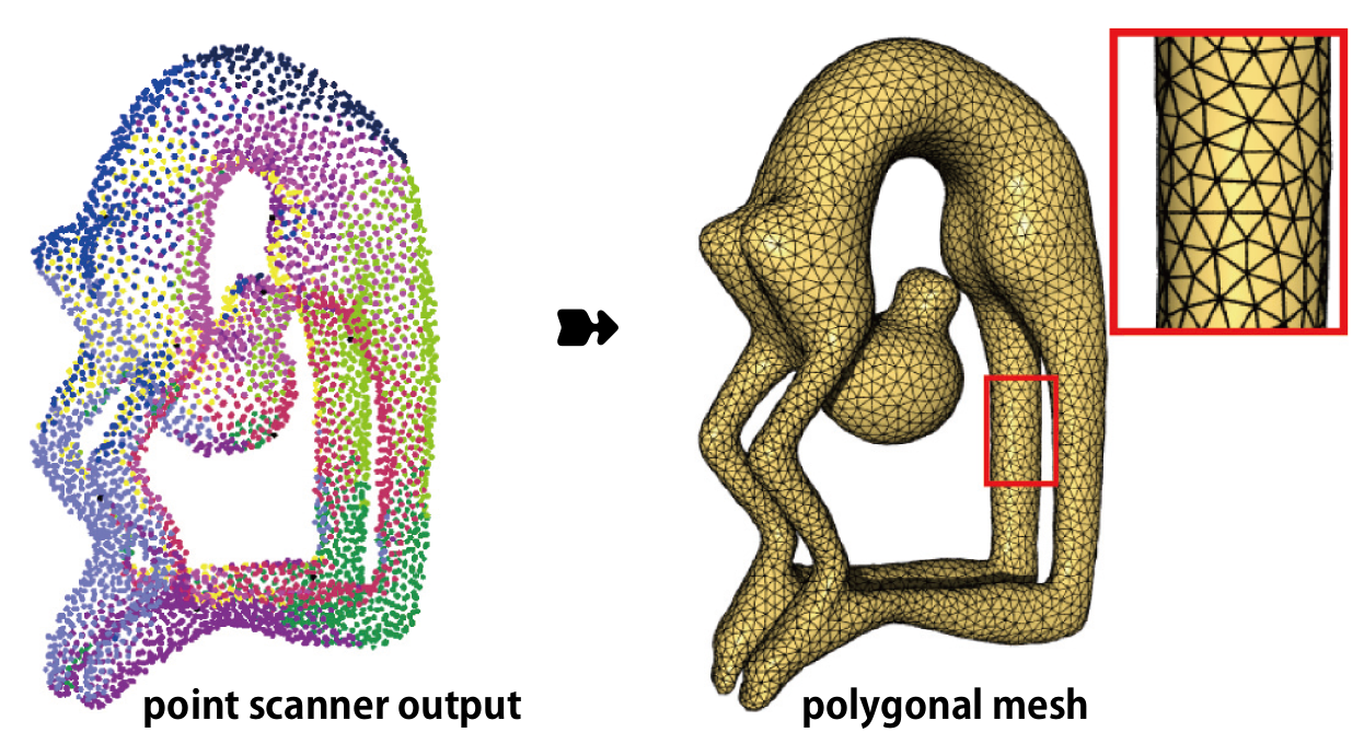
[Diamanti et al., 2023]
In the remainder of this chapter,
we will only focus on the reconstruction step.
[Diamanti et al., 2023]
(You will see, this is a very nice application of Marching Cubes!)
What do you get from a range scan?
- Option 1: only 3D points
- You need to manually estimate the normals
- Can be done by fitting a local tangent plane
(using least squares with the k-nearest points) - This yields rather bad surfaces
- Option 2: points and normal vectors
- You get the normal vectors directly from the range scanner.
Either way, you must have one normal vector for each point, otherwise we cannot reconstruct a surface.
The Core Idea
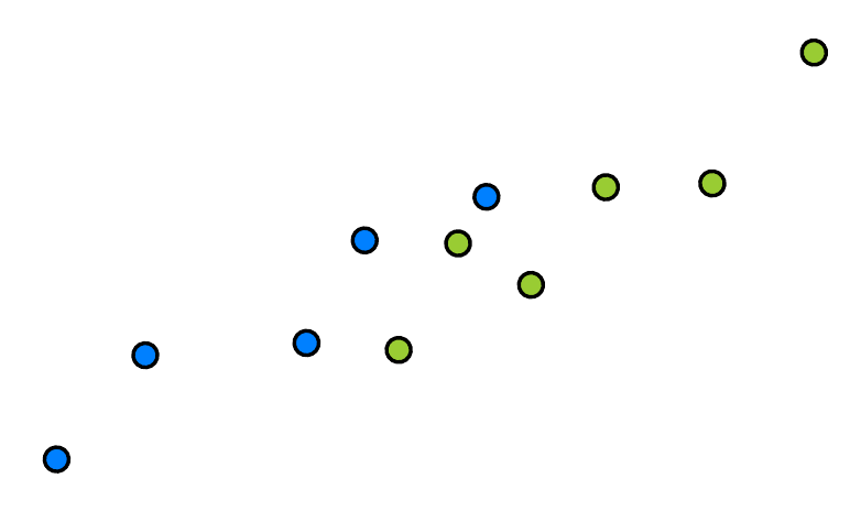
Raw points from the range scan.
$\downarrow$
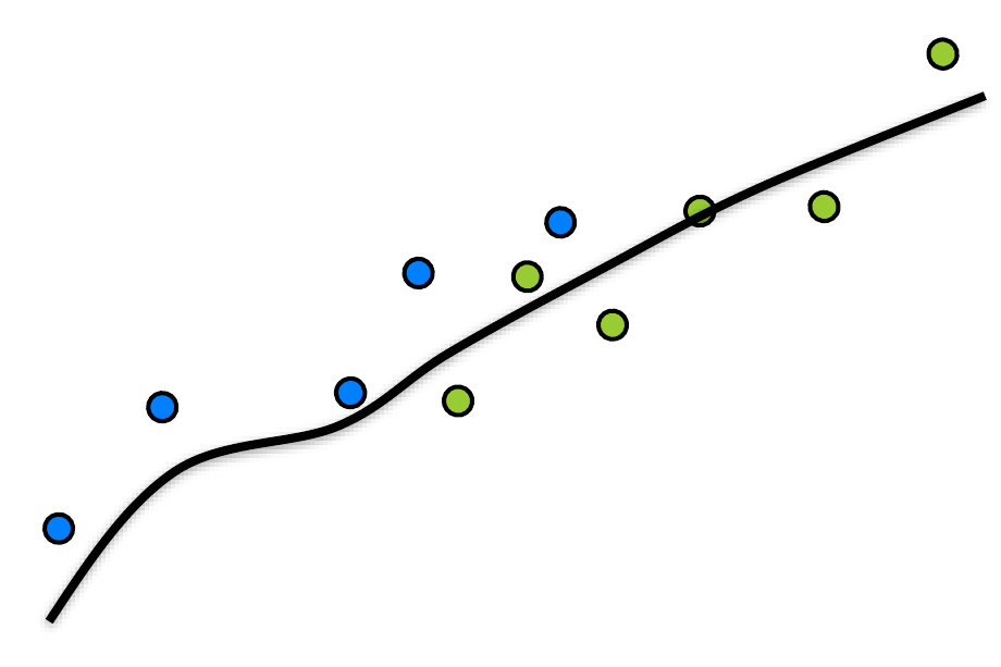
We can fit an SDF to the points.
From the scanner we got points for each scan.
Core Idea: The points are approximately on a 0-level set of a signed distance function.
Using the normals we have a notion of inside and outside.
Figures by [Diamanti et al., 2023]
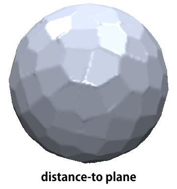
The Naive Approach (1)
Compute signed distance to the tangent plane of the closest point.
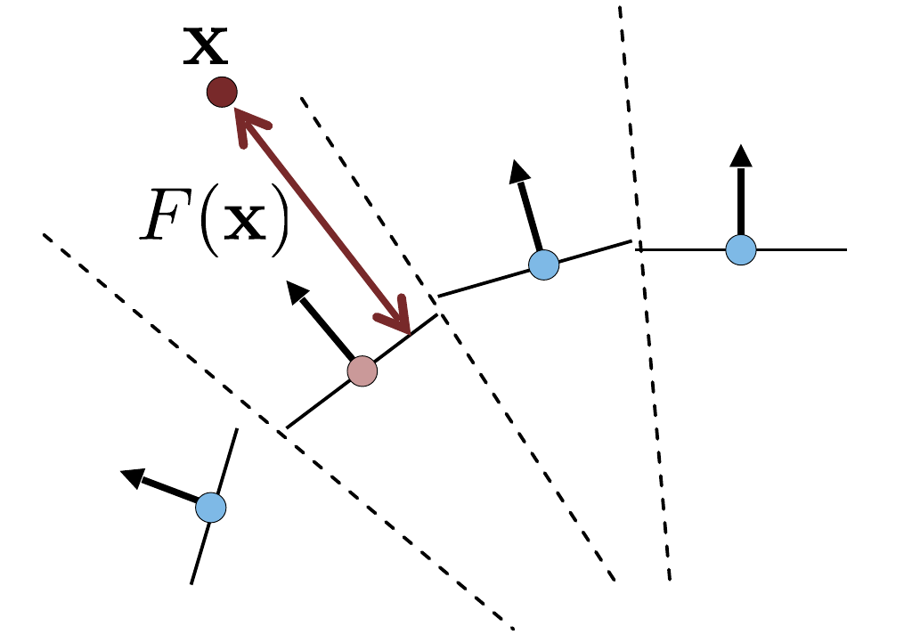
Figures by [Diamanti et al., 2023]
This is a simple approach. For each $x \in \mathbb{R}^3$ we can retrieve the nearest neighbor of the set of scanned points. Using the normal vector of the retrieved scanned point, we can compute the tangent plane. The signed distance is then simply the distance of $x$ to the tangent plane.
So what is the problem with this?
The Naive Approach (2)
The resulting SDF will be discontinuous!
[Diamanti et al., 2023]
Points close to the dashed line will experience sudden jumps.
The resulting mesh would not be smooth.
The Interpolation Problem (1)
To construct an SDF $F$, we will need to solve an approximation/interpolation problem:
\[ F = \argmin_{f \in \mathcal{F}} \sum_{i=1}^N ||f(\mathbf{x}_i) - \hat{F}_i||^2 \]We want to find function $f$ from the space of acceptable functions $\mathcal{F}$ that minimizes the error between any known distance $\hat{F}_i$ at given points $\{\mathbf{x}_i \in \mathbb{R}^3\}$ and the estimated distance value obtained from $f$.
Naturally, this will result in $F \equiv 0$ as the trivial optimal solution; therefore, we need to define constraints.
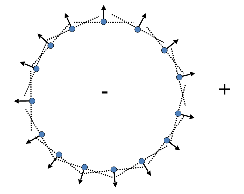
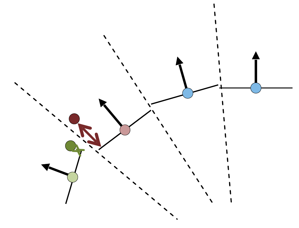
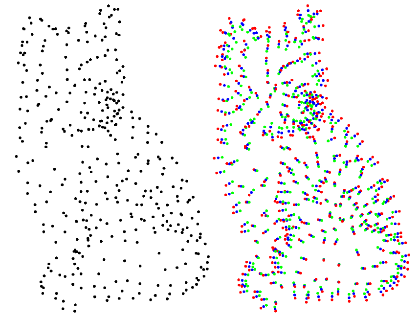
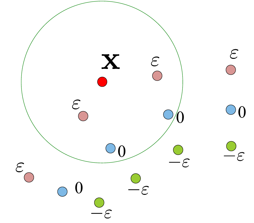
The Interpolation Problem (2)
We now add off-surface constraints for each point $\mathbf{p}_i$ by moving the points along their normals $\mathbf{n}_i$ by some $\varepsilon$
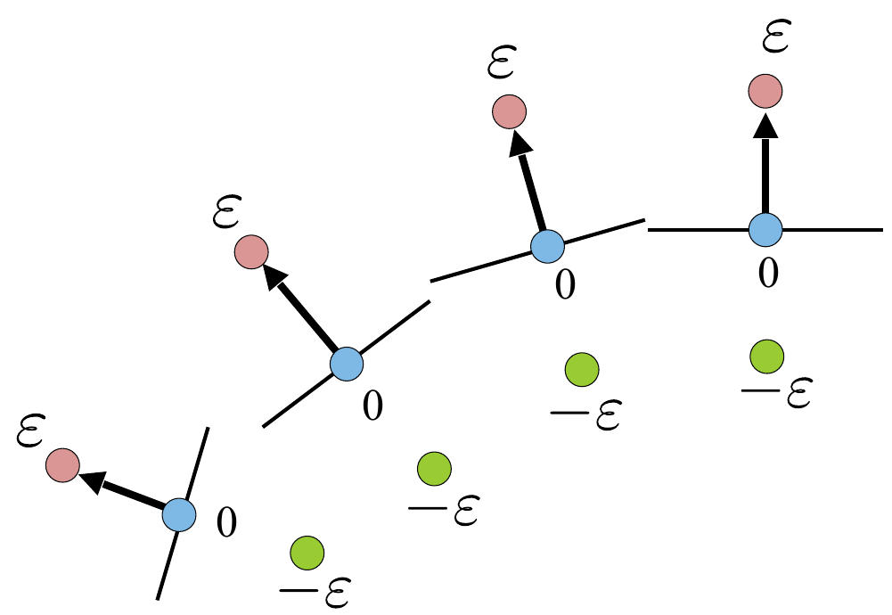
[Diamanti et al., 2023]
- $F(\mathbf{p}_i) = 0$
- $F(\mathbf{p}_i + \varepsilon \mathbf{n}_i) = \varepsilon$
- $F(\mathbf{p}_i - \varepsilon \mathbf{n}_i) = -\varepsilon$
This now defines in total $3n$ equations for the interpolation problem.
The Interpolation Problem (3)
There are two ways to solve the interpolation problem:
Radial Basis Functions
Construct a global linear equation system.
Moving Least Squares
Piecewise solving of smaller equation systems.
Radial Basis Functions (1)
A function $\phi: \mathbb{R}^d \rightarrow \mathbb{R}$ is called radial
if its function value only depends on the magnitude of its argument.
Example: $\phi(\mathbf{x}) = \varphi(||\mathbf{x}||) = \varphi(r)$ where $\varphi: [0, \infty) \rightarrow \mathbb{R}$
$\phi$ is constant for input vectors of the same length.
Radial Basis Functions (2)
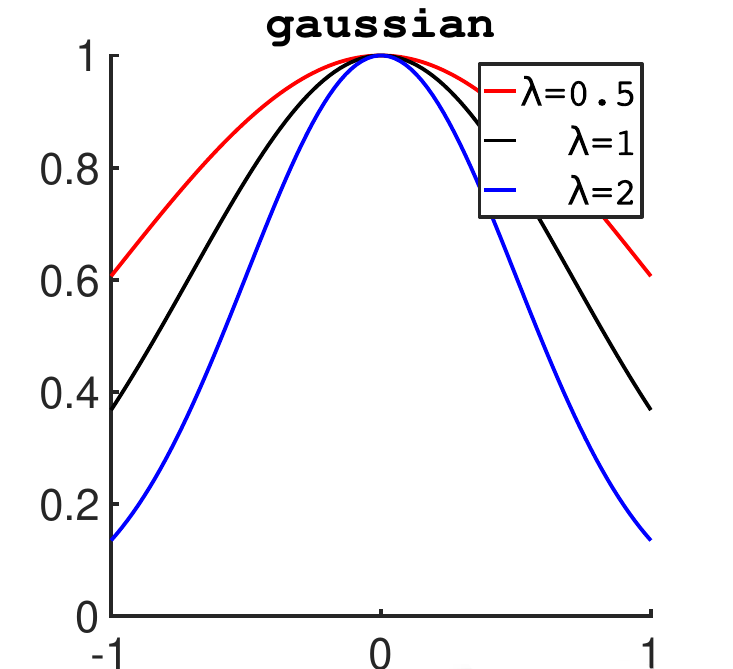
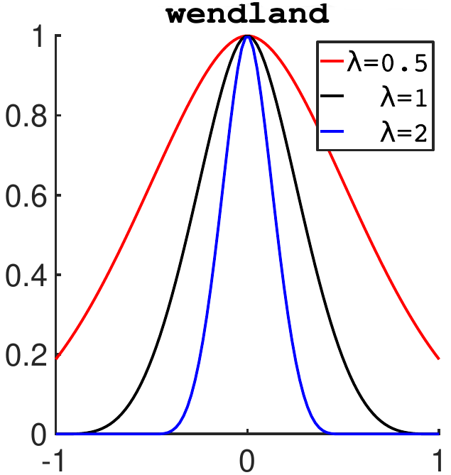
Two prominent examples
The wendland function is frequently used, because it clamps values to zero if they exceed $\lambda$.
Note: Even though the functions in these plots also show a negative domain, the radial basis functions will in general only receive arguments within $[0, \infty)$.
Figures by [Diamanti et al., 2023]
Radial Basis Functions (3)
We can also center a radial basis function at $\mathbf{c}$
\[ \phi_{\mathbf{c}}(\mathbf{x}) = \varphi(||\mathbf{x} - \mathbf{c}||) \]In this case we call $\phi_{\mathbf{c}}$ a radial kernel centered at $\mathbf{c}$
Radial Basis Functions (4)
Our interpolated & approximated SDF will now take the following form:
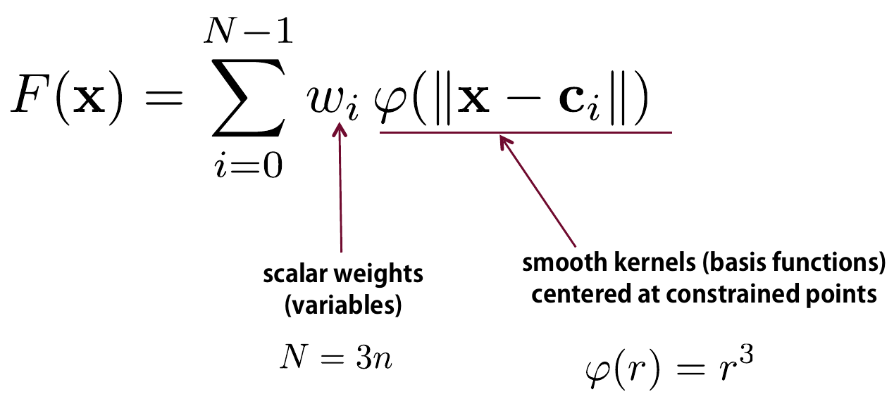
Now we only need to find the weights $w_i$.
Radial Basis Functions (5)
We can now formulate linear equations for a linear system:
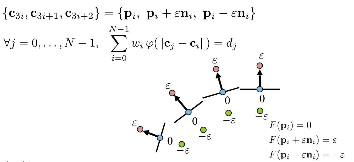
With this system we formulate a distance value of the SDF for every point, including our off-surface points.
Note: $d_j$ is either $0$, $-\varepsilon$ or $\varepsilon$ Figures by [Diamanti et al., 2023]
Radial Basis Functions (6)
The final linear system:
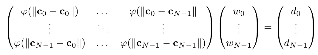
This can be solved by any off-the-shelf solver and yields the weights for our SDF.
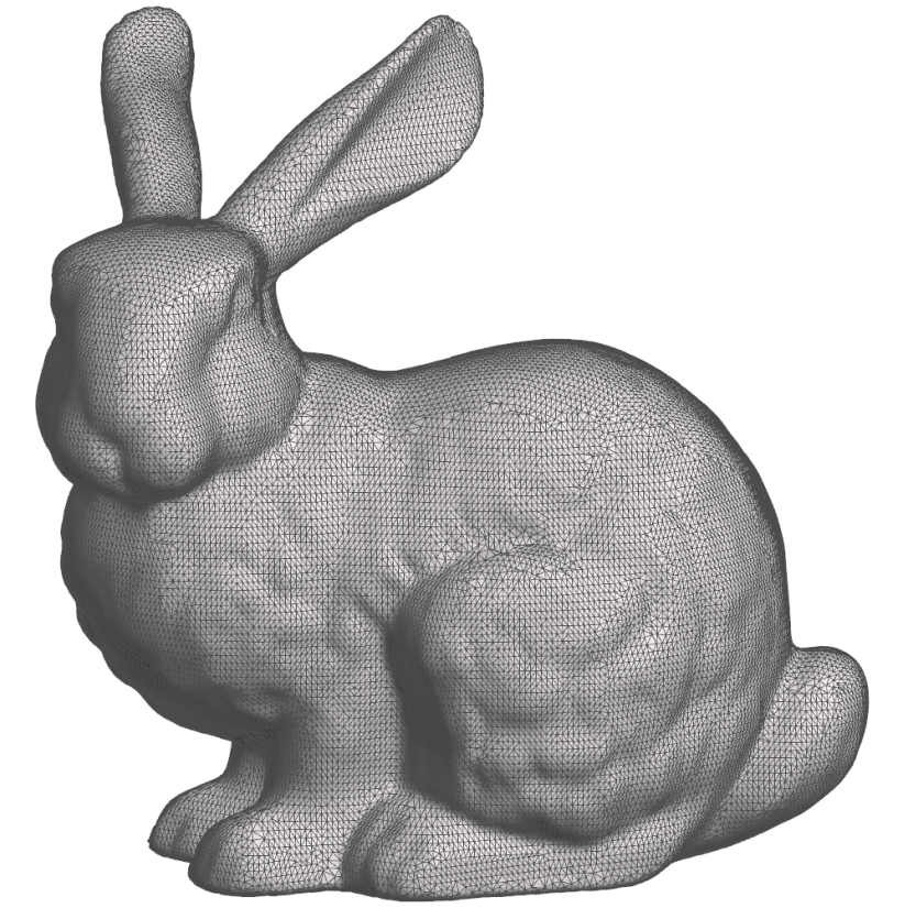
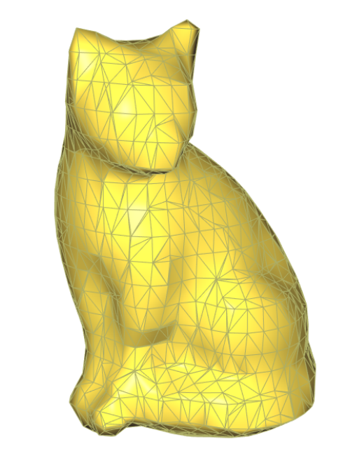
Final Step: Marching Cubes
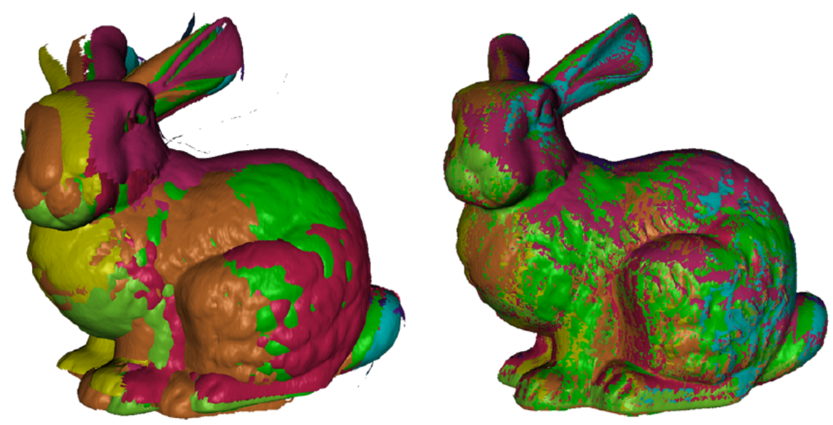
Discussion
The SDF with RBF yields much smoother results than our naive approach.
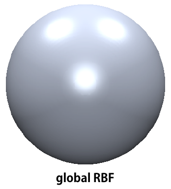
Advantage: Sees the whole data set $\rightarrow$ very smooth surfaces.
Disadvantage: Global (dense) system to solve ‒ expensive.
Moving Least Squares (1)
 [Diamanti et al., 2023]
We would like to approximate a SDF with points in the local vicinity of point $\mathbf{x}$ instead of using the entire dataset. The weights therefore change depending on where we are evaluating.
The "stitching" of all local approximations, seen as one function $F(\mathbf{x})$, is smooth everywhere! We get a globally smooth function from purely local computation.
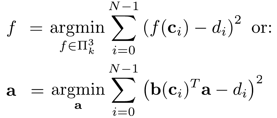
Moving Least Squares (2)
We now compute a polynomial (our SDF) using least-squares. First, choose a degree $k$. Note that the number of points does not determine the form of the polynomial, only the chosen degree k does this.
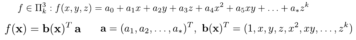
In this polynomial, we now need to find the coefficients $\mathbf{a}$, which minimize the sum of squared differences. Here we now use the points in the local vicinity of $\mathbf{x}$.
Moving Least Squares (3)
The result becomes a lot smoother if we assign more weight to points closer to $\mathbf{x}$. Therefore we now multiply each term with a weight function that takes the distance from $\mathbf{x}$ to the dataset point as input.
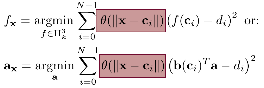
Example weight function:
\[ \theta(r) = e^{-\frac{r^2}{h^2}} \]The value of the SDF at $\mathbf{x}$ is the obtained approximation "from the perspective of $\mathbf{x}$":
\[ F(\mathbf{x}) = f_{\mathbf{x}}(\mathbf{x}) = b(\mathbf{x})^T \mathbf{a}_\mathbf{x} \]The MLS function $F$ is continuously differentiable if and only if the weight function $\theta$ is continuously differentiable.
Discussion
RBF yields better results, but MLS is much less expensive to compute!
RBF
Advantage:
Sees the whole data set $\rightarrow$ very smooth surfaces.
Disadvantage:
Global (dense) system to solve ‒ expensive.
MLS
Advantage:
local linear solves ‒ cheap
Disadvantage:
sees only a small part of the dataset, can get confused by noise.
Outlook
Why did I show you all this?
Reconstructing an explicit surface from a raw set of points is a
core geometry processing task.
The pipeline is a beautiful interplay between SDF and Marching Cubes and shows you:
Results by Marching Cubes depend on designing a good SDF.
There are many ways to improve marching squares / cubes!
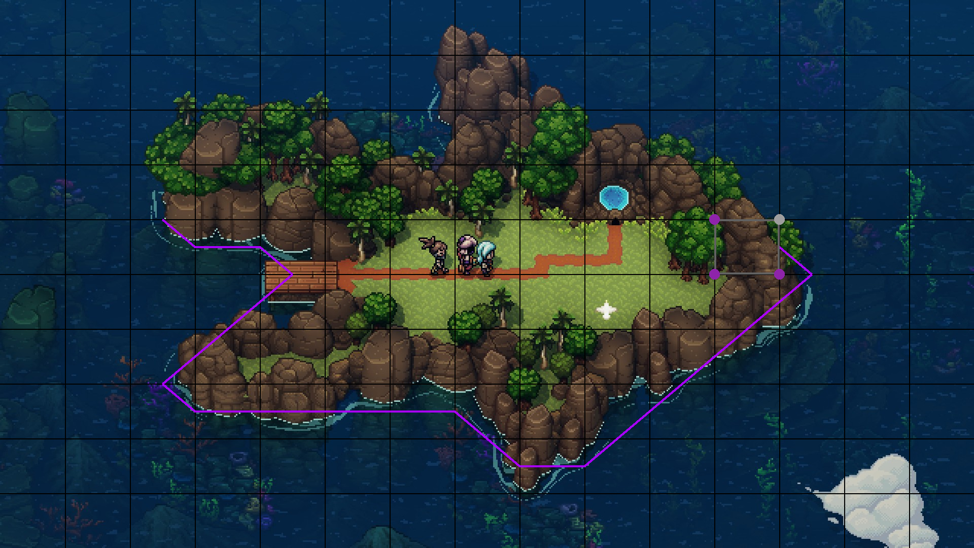
A sailor would simply
sail around the island.
The Marching Alternative: Tracking
Instead of iterating the entire grid, we could also simply track the contour through neighboring cells.
Edge tracking on our beloved island.
Iteration 0

Iteration 1

Iteration 2
Iteration 23
Iteration 37
Iteration 43
In 3D we would "grow" a surface
[A.Hilton & J.Illingworth (1997). Marching Triangles: Delaunay Implicit Surface Triangulation.]
This also allows us to adjust the triangle size to local curvature.
Edge Tracking is a more sophisticated way of marching the grid.
Advantage: Performance improvement.
Caveat: You need one seed cell for each component.
Hints on the Exam
Four types of questions are possible:
- Explain a concept, e.g. how does Marching Cubes work.
Yes, you should also know how the heavy math works. But you won't need a calculator. - Answer questions about the specific intricacies, e.g. ambiguities.
Usually these will be single choice questions. - Apply concepts of the Marching Cubes algorithm.
- Transfer the Marching Cubes algorithm to a new situation.