How to read these slides?


 Overview
Click on the menu bar items to navigate to chapters
Click here for PDF version

Constrained Functions
Functional Data Analysis - Chapter 6
CEDAS FDA-VDS Seminar 2026
Julian Rakuschek
11.06.2026
In this lecture
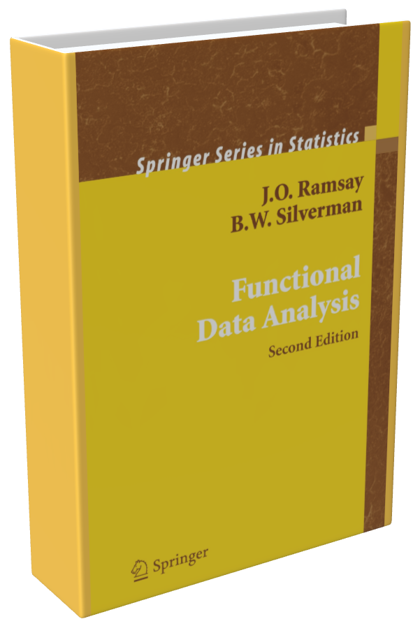
We are going to cover chapter 6 in Functional Data Analysis on Constrained Functions
Focus:
- Positive functions
- Monotonically increasing functions
- Probability density function estimation
Positive Functions
Which functions are positive? (1 / 3)
Counts, for example page views
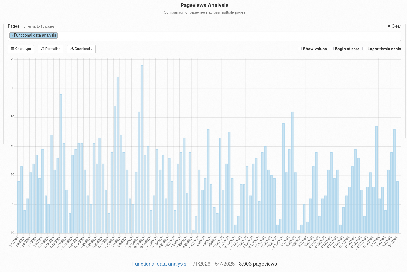
Strictly speaking: This would be non-negative
Which functions are positive? (2 / 3)
Probability functions
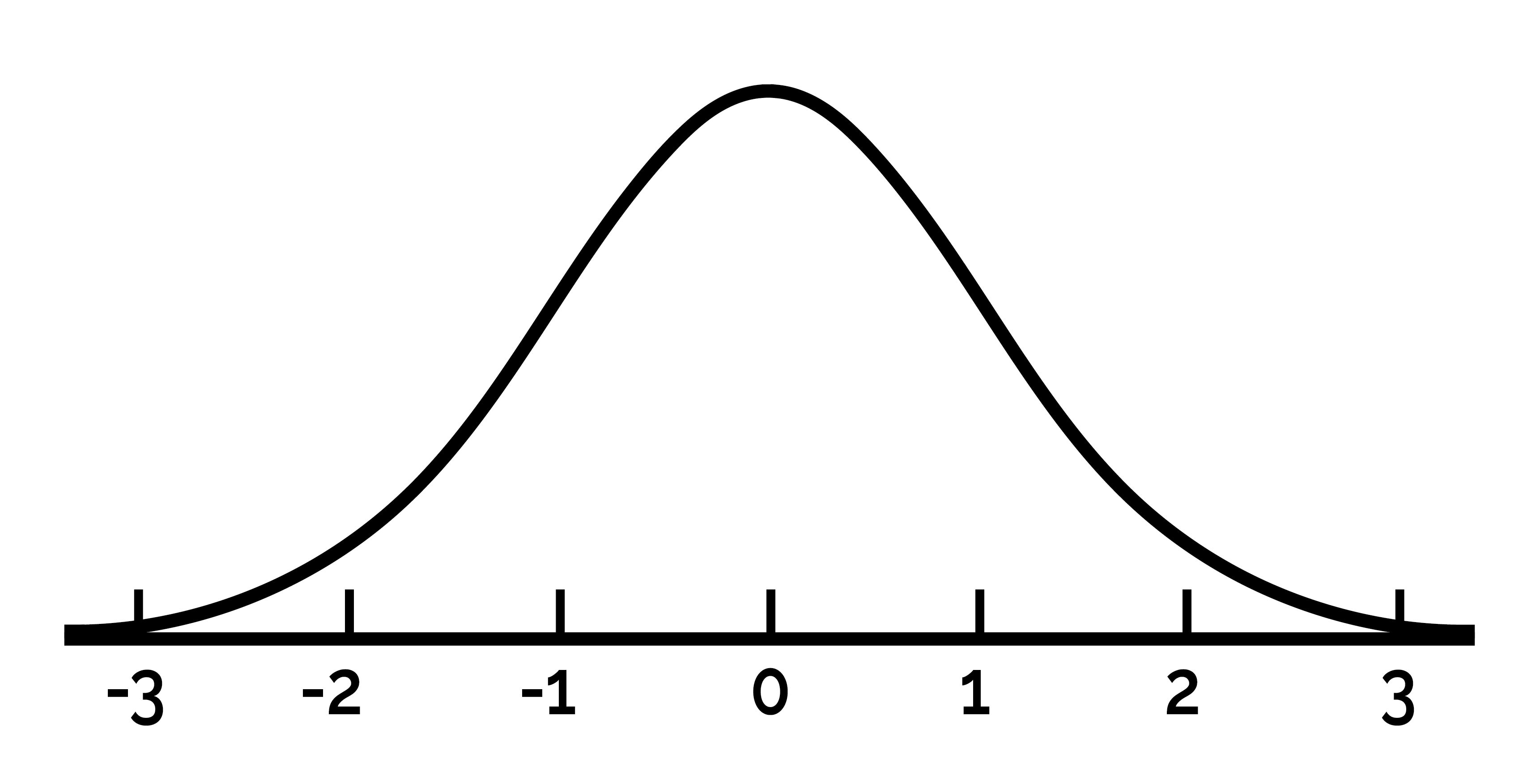
Which functions are positive? (3 / 3)
Many quantities can only be positive
Energy
- Kinetic Energy
- Potential Energy
Measures
- Area
- Volume
- Length
Information Theoretic
- Entropy
- Mutual information
- Divergences
Pinch Force
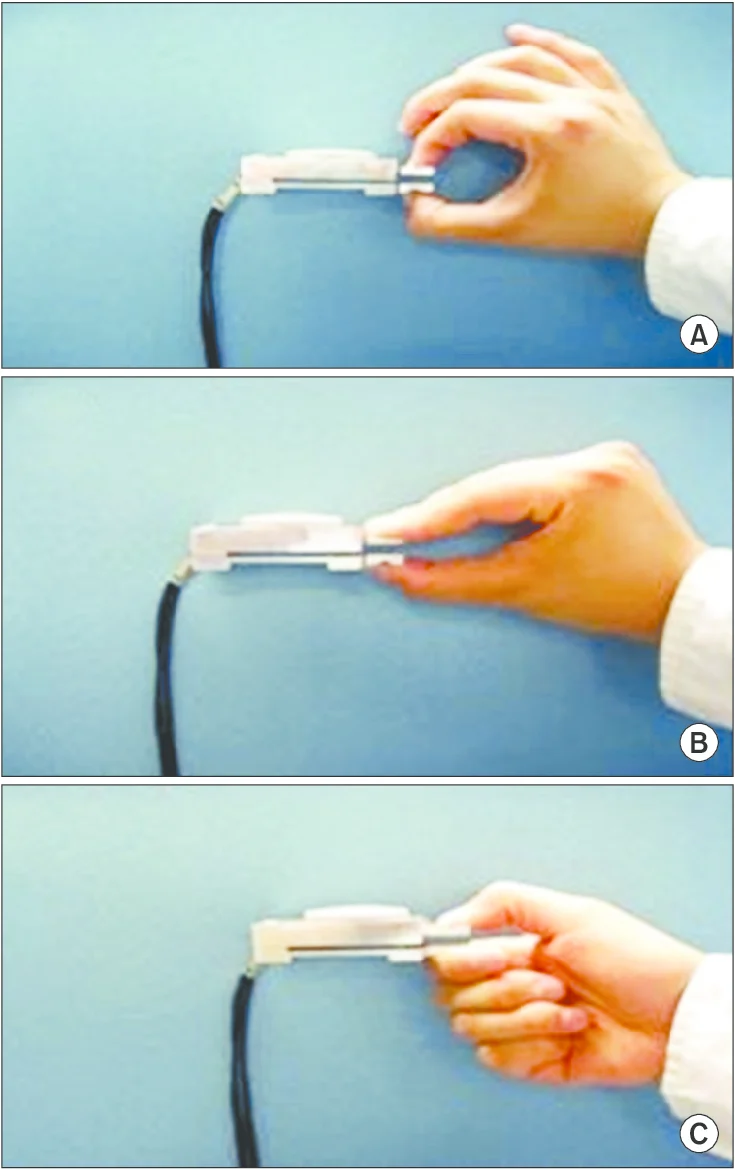
Image Source: Kong, Sangwon & Lee, Kyung & Kim, Junho & Jang, Seong. (2014). The Effect of Two Different Hand Exercises on Grip Strength, Forearm Circumference, and Vascular Maturation in Patients Who Underwent Arteriovenous Fistula Surgery. Annals of Rehabilitation Medicine. 38. 648. 10.5535/arm.2014.38.5.648.
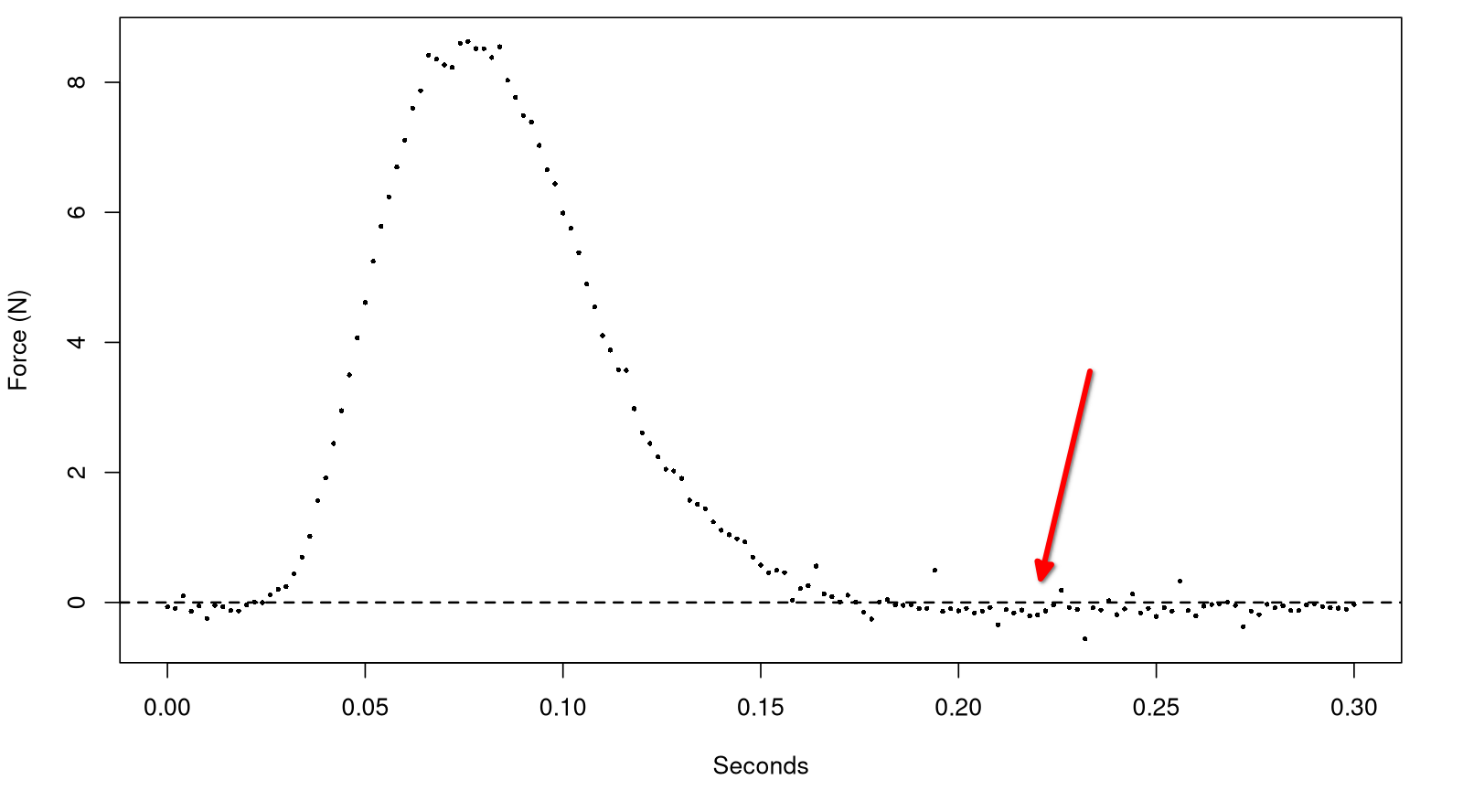
Measurements can be noisy and drop below zero
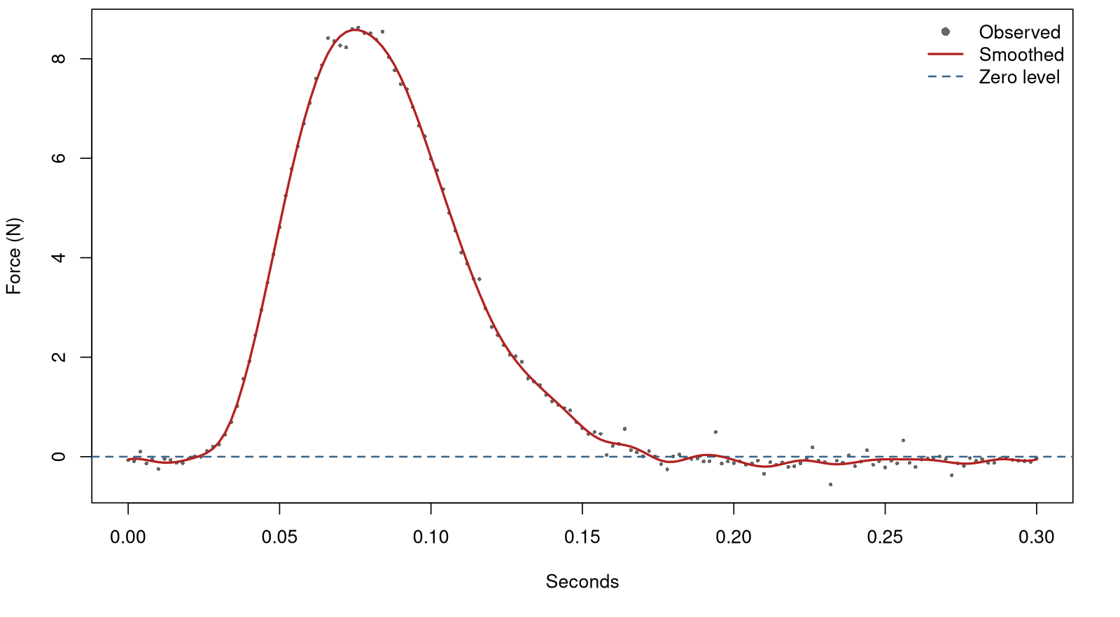
The way we have fitted a function previously
Chapter 5 – smoothing with roughness penalty:
\[ \text{PENSSE}_\lambda(x|\mathbf{y}) = \underbrace{[\mathbf{y}-x(\mathbf{t})]^T \mathbf{W} [\mathbf{y}-x(\mathbf{t})]^2}_{\text{Fit of the data}} + \lambda \underbrace{\int (D^2 x(s))^2 ds}_{\text{Function roughness based on curvature}} \]Remember, $x(t)$ is a linear expansion
\[ x(t) = \sum_{k=1}^K c_k \phi_k (t) \]In the FDA package
fdParobj <- fdPar(
    fdobj = basis,
    Lfdobj = 2,
    lambda = 1e-8
)

fit <- smooth.basis(
    argvals = x_values,
    y = y_values,
    fdParobj = fdParobj
)
This creates some noisy tails
Defining positive smoothing functions
Instead of
\[ x(t) = \sum_{k=1}^K c_k \phi_k (t) \]we now define
\[ x(t) = e^{\sum_{k=1}^K c_k \phi_k (t)} = e^{W(t)} \]Positive smoothing function $x$ can always be defined on the exponential of an unconstrained function $W$.
Remarks
\[ x(t) = e^{W(t)} \]Any other basis can be used as well!
Nota bene: This function can never be exactly zero. It can only get very close to zero.
The updated optimization criterion
\[ \text{PENSSE}_\lambda(x|\mathbf{y}) = [\mathbf{y}-x(\mathbf{t})]^T \mathbf{W} [\mathbf{y}-x(\mathbf{t})]^2 + \lambda \int (D^2 x(s))^2 ds \]now becomes
\[ \text{PENSSE}_\lambda(\textcolor{red}{W}|\mathbf{y}) = [\mathbf{y}-\textcolor{red}{e^{W(\mathbf{t})}}]^T \mathbf{W} [\mathbf{y}-\textcolor{red}{e^{W(\mathbf{t})}}]^2 + \lambda \int (D^2 \textcolor{red}{W(t)})^2 dt \]Needs to be solved through numerical methods. But these converge quickly because the expression is only mildly nonlinear.
smooth.basis $\rightarrow$ smooth.pos
fdParobj <- fdPar(
    fdobj = basis,
    Lfdobj = 2,
    lambda = 1e-8
)

fit <- smooth.pos(
    argvals = x_values,
    y = y_values,
    WfdParobj = fdParobj,
    dbglev = 0
)
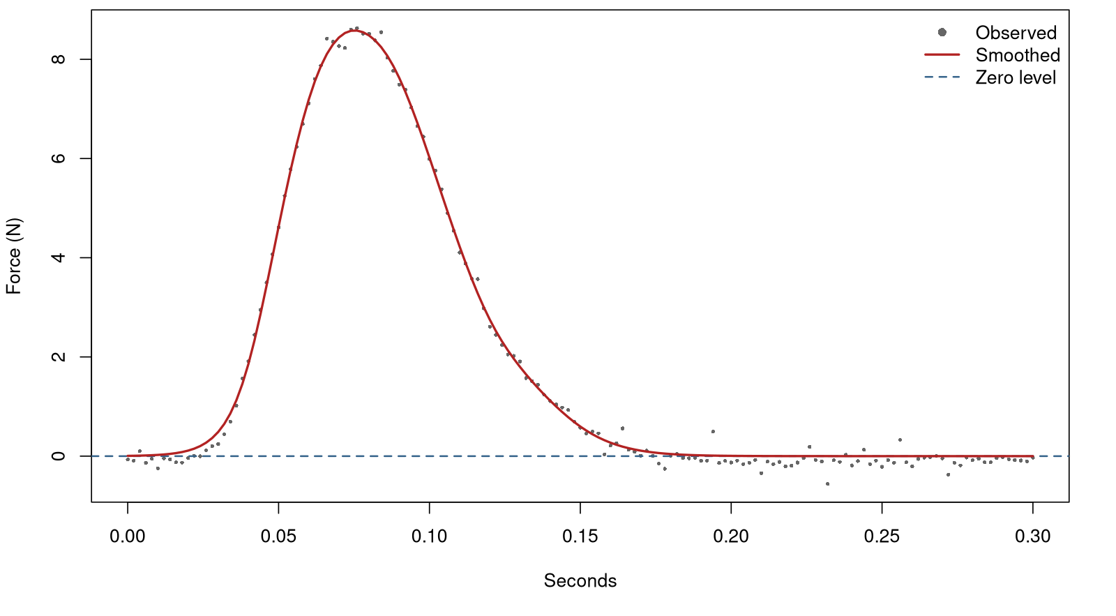
Comparison
Unconstrained
Constrained
Monotone Functions
Which functions are monotone? (1 / 3)
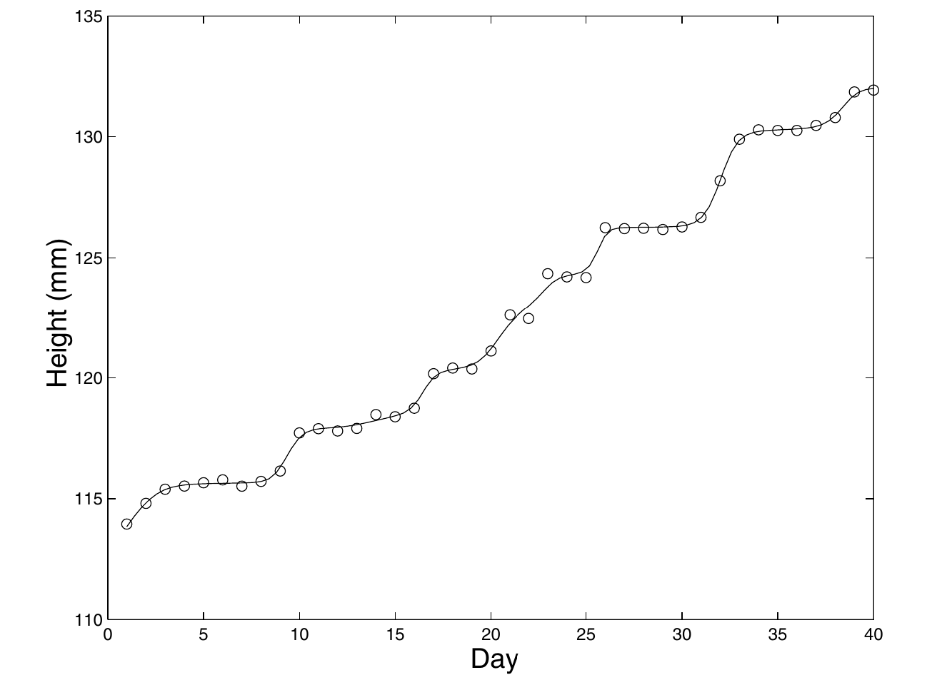
Growth
Which functions are monotone? (2 / 3)
Growth
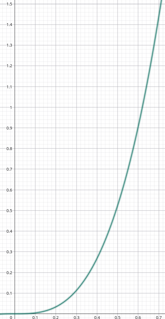
Volume is monotone increasing in the radius.
\[ V(r) = \frac{4}{3} \pi r^3 \]Which functions are monotone? (3 / 3)
Cumulative Distribution Functions
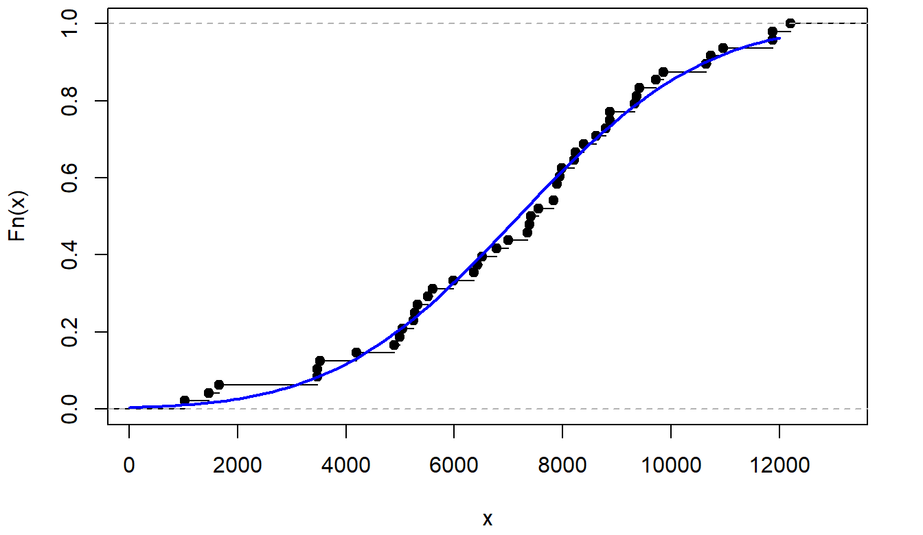
The Tibia Dataset
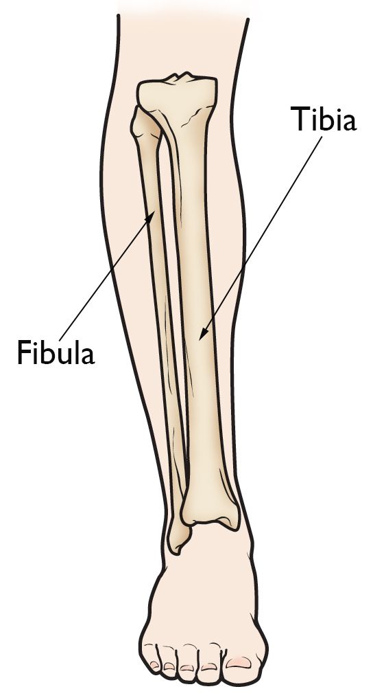
Fitting with the previous approach
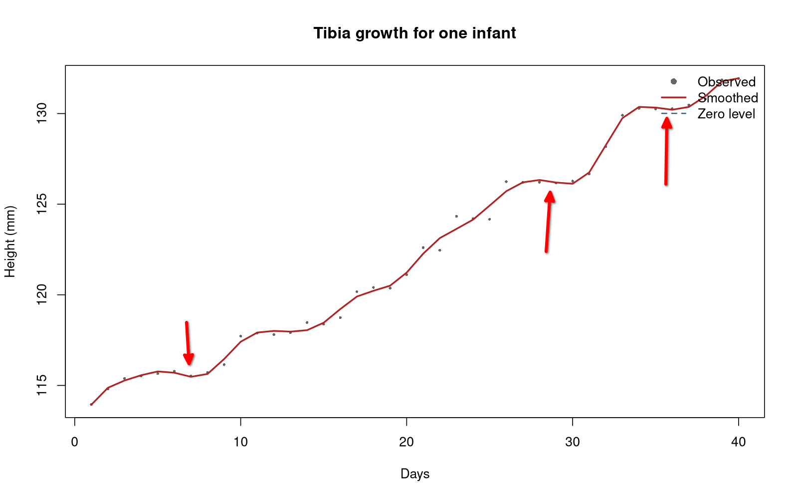
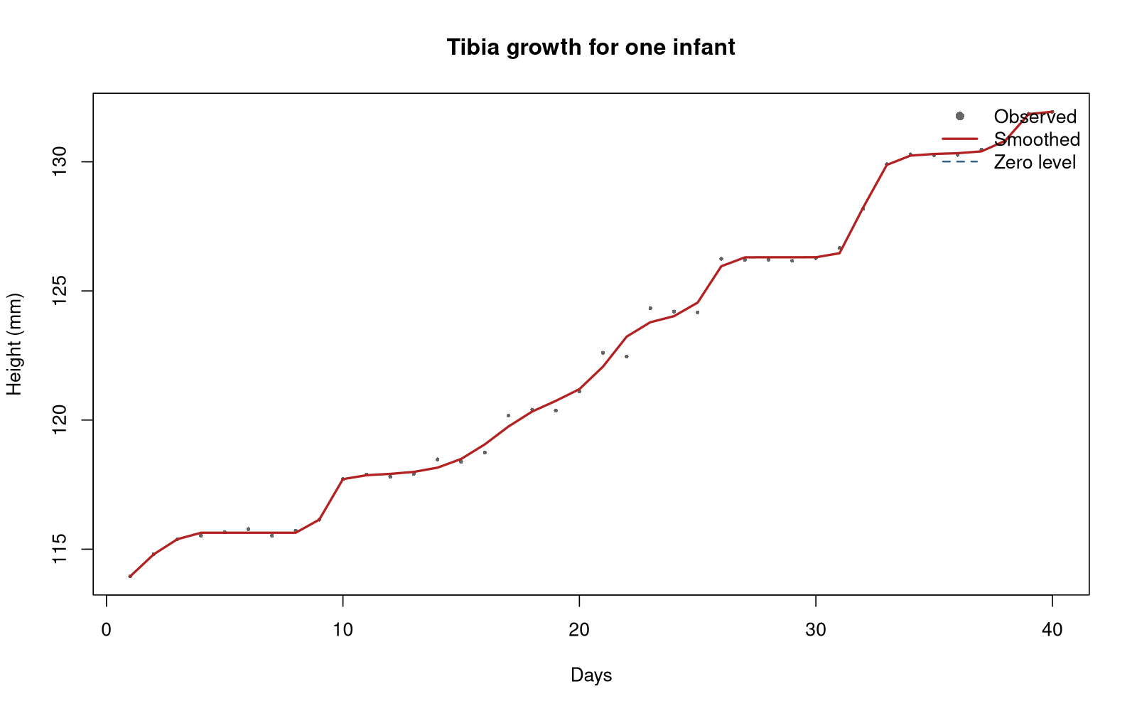
Ensuring monotone behavior
The first derivative must be positive everywhere.
\[ Dx(t) = e^{W(t)} \] Integrate both sides: \[ x(t) = c + \int_{t_0}^t e^{W(u)} du \]$c$ is a constant estimated from the data.
Depending on $c$, the function will also be positive everywhere once it crosses the 0-level.
But: A zero increase is not possible, the function is always strictly monotone.
The updated optimization criterion
\[ \text{PENSSE}_\lambda(x|\mathbf{y}) = [\mathbf{y}-x(\mathbf{t})]^T \mathbf{W} [\mathbf{y}-x(\mathbf{t})]^2 + \lambda \int (D^2 x(s))^2 ds \]now becomes
\[ \text{PENSSE}_\lambda(\textcolor{red}{W}|\mathbf{y}) = \\ \left[\mathbf{y}-\textcolor{red}{\left(c + \int_{t_0}^t e^{W(u)} du\right)}\right]^T \mathbf{W} \left[\mathbf{y}-\textcolor{red}{\left(c + \int_{t_0}^t e^{W(u)} du\right)}\right]^2 \\ + \lambda \int (D^2 \textcolor{red}{W(t)})^2 dt \]Needs to be solved through numerical methods.
smooth.basis $\rightarrow$ smooth.monotone
fdParobj <- fdPar(
    fdobj = basis,
    Lfdobj = 2,
    lambda = 1e-8
)

fit <- smooth.monotone(
    argvals = x_values,
    y = y_values,
    WfdParobj = fdParobj
)
Comparison
Unconstrained
Constrained
Probability Density Functions
We now want to fit a probability density function
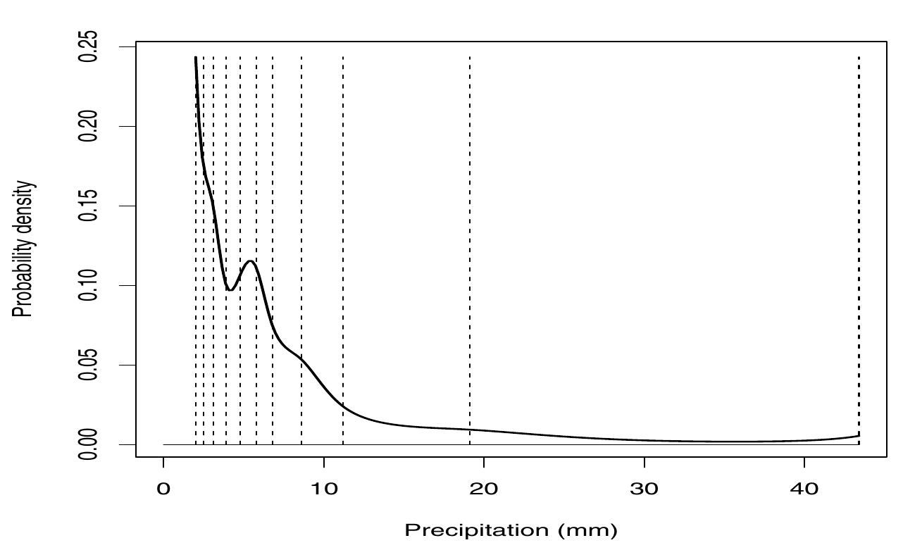
Each $t$ has a probability of $p(t)$ to occur.
Two constraints for this function
\[ \Large p(t) > 0 \\ \int p(t) dt = 1 \]$p(t)$ therefore looks like this:
This is our density model.
Remember our basis expansion
\[ W(t) = \sum_{k=1}^K c_k \phi_k (t) \]The goal is to find an optimal coefficient vector $c$ for the model $p(t) = \frac{e^{W(t)}}{\int e^{W(t)} dt}$
Using maximum likelihood estimation is the way to go!
Likelihood Refresher
Likelihood for all $N$ observations $t_1, \ldots, t_N$:
\[ L(W|c) = \prod_{i=1}^N p(t_i) \]Maximum likelihood means finding a density that assigns high probability density to the observed samples.
Products are annoying
Therefore we apply the log to convert it to a sum:
\[ \log L(W|c) = \sum_{i = 1}^N \log p(t_i) \]Insert our density model
\[ \log L(W|c) = \sum_{i = 1}^N \log p(t_i) = \sum_{i = 1}^N \log \left( \frac{e^{W(t)}}{\int e^{W(t)} dt} \right) \]Apply $\log \left( \frac{A}{B} \right) = \log A - \log B$
\[ = \sum_{i = 1}^N \left[ \log \left(e^{W(t)}\right) - \log \left( \int e^{W(t)} dt \right) \right] \\ = \sum_{i = 1}^N \left[ W(t) \right] - N \log \left( \int e^{W(t)} dt \right) \]Insert basis expansion
\[ \log L(W|c) = \sum_{i = 1}^N \left[ \textcolor{red}{\mathbf{c}^T \phi(t_i)} \right] - N \ln \left( \int e^{\textcolor{red}{\mathbf{c}^T \phi(t_i)}} dt \right) \]So what do the terms mean?
\[ \log L(W|c) = \sum_{i = 1}^N \left[ \mathbf{c}^T \phi(t_i) \right] - N \ln \left( \int e^{\mathbf{c}^T \phi(t_i)} dt \right) \]the term forces the density to integrate to $1$.
Let's apply this to the R galaxies dataset!
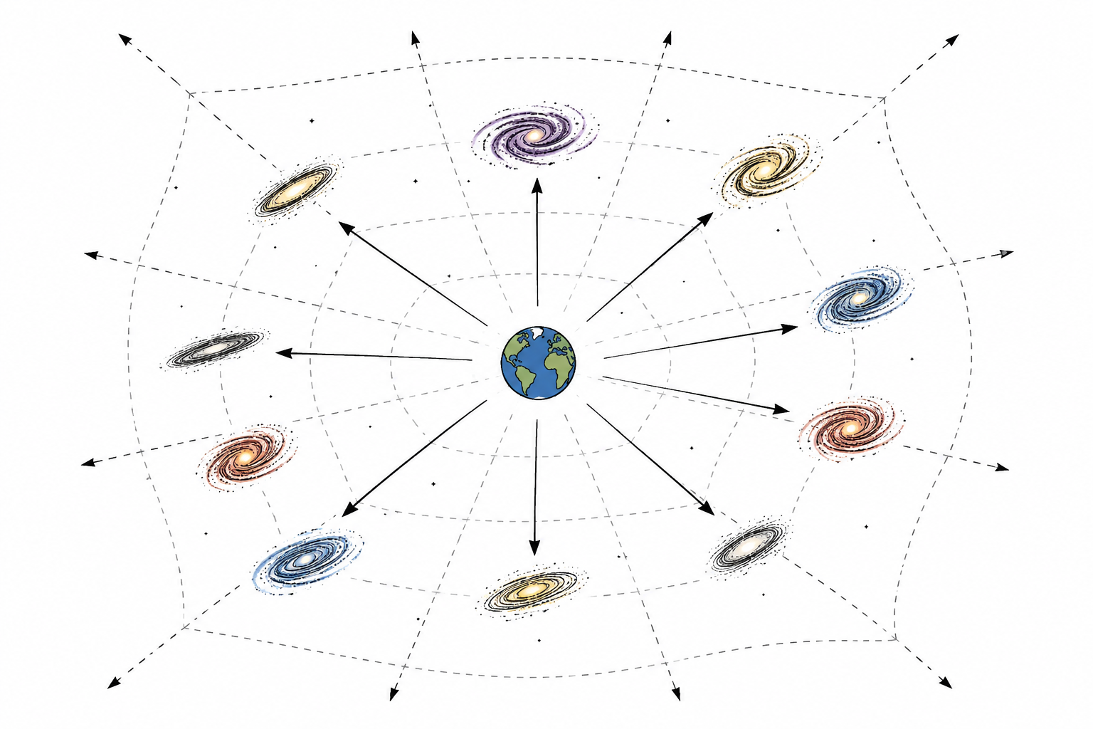
82 observatons of the velocities (in 1000 km/second) of distant galaxies diverging from our own
The dataset is a simple list of velocities

Constructing the R script (1)
Preliminaries
library(fda)
library(MASS)
data(galaxies)
dataset <- galaxies
N <- length(dataset)
Constructing the R script (2)
Construct a B-Spline basis
Wknots <- dataset[round(N * seq(1 / N, 1, length.out = 11), 0)]
Wnbasis <- length(Wknots) + 2
Wbasis <- create.bspline.basis(
  rangeval = range(dataset),
  nbasis   = Wnbasis,
  norder   = 4,
  breaks   = Wknots
)
Constructing the R script (3)
Then we compute the fit using density.fd
Wlambda <- 0
Wfd0 <- fd(matrix(0, Wnbasis, 1), Wbasis)
WfdPar <- fdPar(Wfd0, Lfdobj = 2, lambda = Wlambda)

# Fit the density with density.fd.
# The result contains:
# - Wfdobj: fitted log-density component W(x)
# - C: normalizing constant
densityList <- density.fd(dataset, WfdPar)
Attention: density.fd is only available up until version 6.2.0. It has been removed in version 6.3.0.
Constructing the R script (4)
Evaluate the fitted fda density on a fine grid.
Wfd <- densityList$Wfdobj
Cconst <- densityList$C
Zfine <- seq(min(dataset), max(dataset), length.out = 401)
Wfine <- eval.fd(Zfine, Wfd)
Pfine <- exp(Wfine) / Cconst
densityList only gives you $W(t)$ and the normalization constant, but not $p(t)$, so you need to stitch it together yourself.
Constructing the R script (5)
Finally plot it.
plot(
  Zfine, Pfine,
  type = "l",
  lwd = 2,
  xlab = "Velocity of galaxy moving away from Earth (km/s divided by 1000)",
  ylab = "Estimated density",
  main = "Galaxy Dataset: density.fd vs KDE"
)

lines(kde_fit$x, kde_fit$y, lwd = 2, lty = 2)
The initial approach overfits badly!
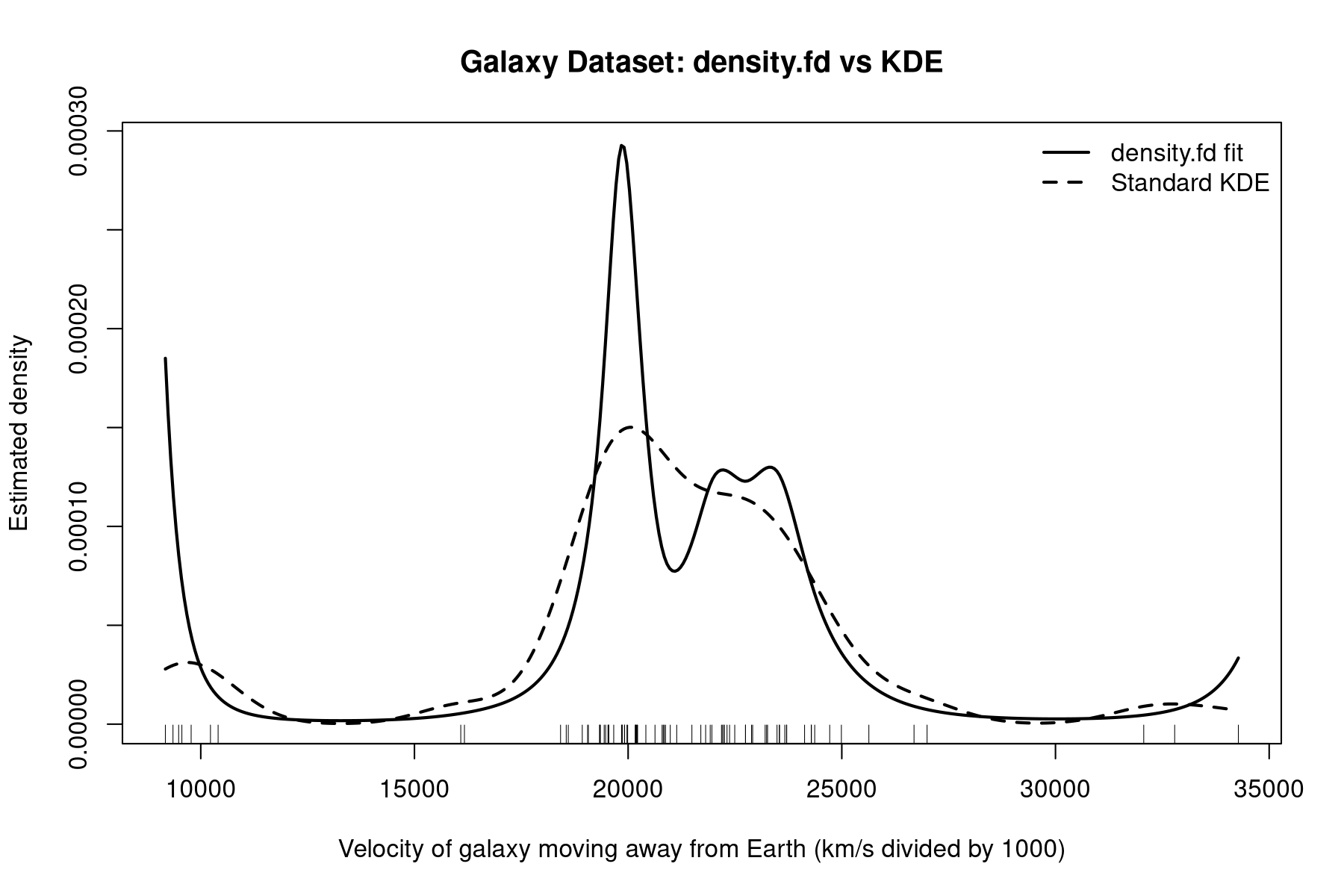
No smoothness control!
Let's extend it with a roughness penalty
\[ \log L(W|c) = \sum_{i = 1}^N \left[ \mathbf{c}^T \phi(t_i) \right] - N \ln \left( \int e^{\mathbf{c}^T \phi(t_i)} dt \right) - \underbrace{ \textcolor{red}{ \lambda \int \left[ D^3 (\mathbf{c}^T \phi(t_i)) \right]^2 dt } }_{\text{PEN}_3(W)} \]$\text{PEN}_3(W)$ penalizes changes in curvature:
- less wiggles
- less oscillations
- less rapid shape changes
$\lambda$ is the smoothing parameter (similar to bandwidth in KDE).
Find coefficient vector $\mathbf{c}$ via numerical optimization.
The density.fd function accepts $\lambda$ as a parameter.
Adjust Wlambda accordingly
Wlambda <- 3e+9
Wfd0 <- fd(matrix(0, Wnbasis, 1), Wbasis)
WfdPar <- fdPar(Wfd0, Lfdobj = 2, lambda = Wlambda)

# Fit the density with density.fd.
# The result contains:
# - Wfdobj: fitted log-density component W(x)
# - C: normalizing constant
densityList <- density.fd(dataset, WfdPar)
The effect of $\lambda$
$\lambda = 0$
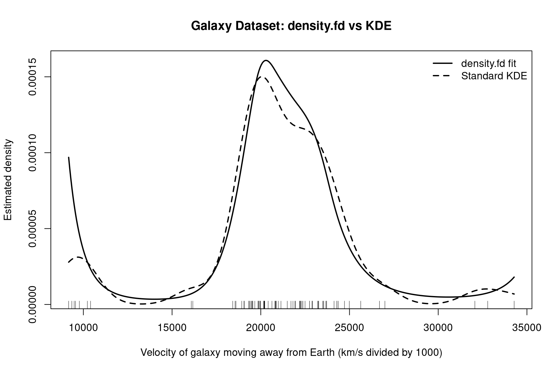
$\lambda = 3 \times 10^9$
For the fda package version 6.3.0, intensity.fd can be used
intensity.fd is essentially the same as density.fd, but does not normalize.
# Fit the intensity with intensity.fd.
# The result contains:
# - Wfdobj: fitted log-intensity component W(x)
densityList <- intensity.fd(dataset, WfdPar)

Wfd <- densityList$Wfdobj

# Evaluate the fitted intensity on a fine grid.
Zfine <- seq(min(dataset), max(dataset), length.out = 401)
Wfine <- eval.fd(Zfine, Wfd)
Ifine <- as.numeric(exp(Wfine))
Same curve, but not normalized.
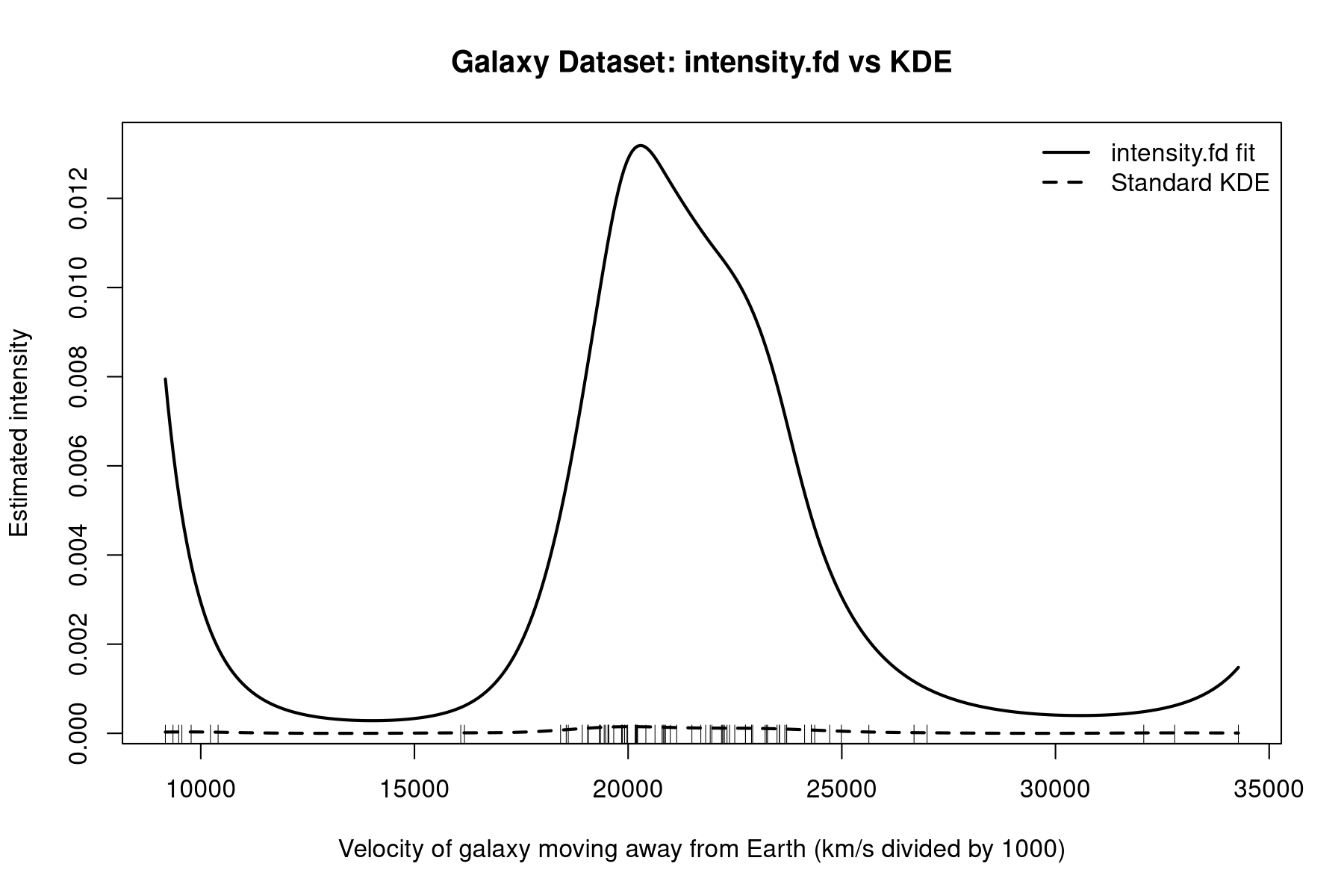
intensity.fd does not provide us a normalization constant.
Extension with weighted samples
Given is weight vector $\mathbf{\omega}$ where $|\omega| = N$
\[ \log L(W|c) =\\ \sum_{i = 1}^N \left[ \textcolor{red}{\omega_i} (\mathbf{c}^T \phi(t_i)) \right] - \textcolor{red}{\left[\sum_{i = 1}^N \omega_i \right]}\ln \left( \int e^{\mathbf{c}^T \phi(t_i)} dt \right) - \lambda \int \left[ D^3 (\mathbf{c}^T \phi(t_i)) \right]^2 dt \]Question to the experts here:
Why would we use this method instead of simply computing the usual KDE?
Exercise

Task in R: Density Estimation
Perform a density estimation on the galaxies dataset!
Open the script density_estimation.r and complete the TODOs.